Updates to Google Sheets
I practiced Lesson 3 by implementing its Excel and Python parts in Google Sheets, I’m documenting here the experiments in case anyone is interested in tweaking some parameters and learning rates and see some plots reflecting those tweaks.
It is a also a resource in case anyone is interested in applying gradient descent with Google Sheets functions and try to fit a linear regression, a quadratic or the sum of 2 Rectified Linear Units (ReLU).
I agree that it is probably more useful to replicate these techniques with Python. The functions in Google Sheets may be getting a little big in order to achieve one iteration in one line. The reality is that the large functions (for loss and partial derivatives) are not written in one shot, they take multiple steps that are then grouped to avoid intermediate references. So they seem more complex that they are to create.
Anyway, the reason to publish this file and this post is based on the probability that they may become useful for someone at some point.
Google Sheets file:
Sheets in the Google Sheets file:
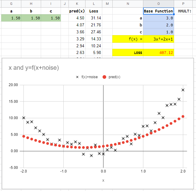
Quadratic Manual
In the “Quadratic Manual” sheet you can manually change the green values for a, b, c. We need to change them to minimize the Loss. We can also see the plot of how the predictions get close to the points generated (those points are created by a base function and some noise added).
You can also change the base function (in this case 3x²+2x+1) by changing the blue a, b, c values.
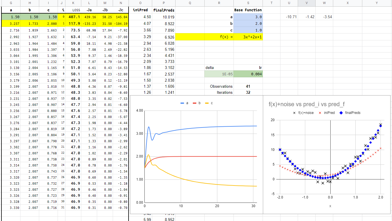
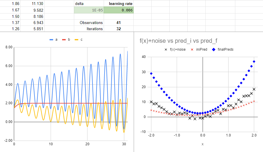
Quadratic GD
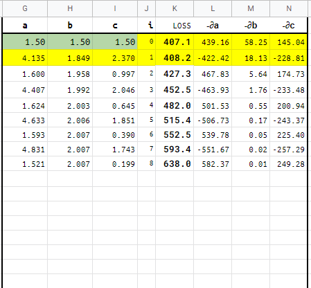
This sheet applies Gradient Descend to automatically find the values a, b, c that best fit the data points (base function + noise).
One plot shows how the parameters a, b and c change in each iteration.
The other has the data points, the first prediction (quadratic with first approximation to parameters) and the quadratic with the final iteration (blue squares predictions).
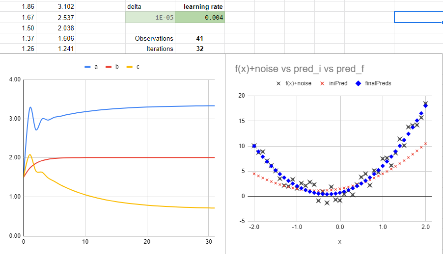
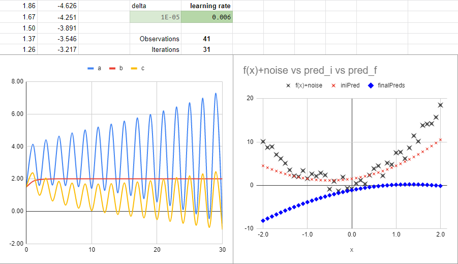
It is interesting to see the difference by changing the learning rate from 0.004
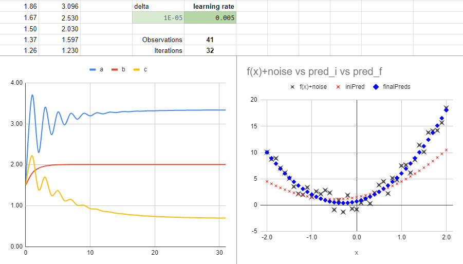
to 0.005
With a learning rate of 0.006 the model doesn’t converge to find the parameters.
We can see how a big learning rate makes the big jumps of parameters a and c, between the values that produces the minimum loss, without the precision to reach that minimum. So, if we delete the last iteration, we can see how the predictions are jumping between the result.
To add or delete iterations, use copy and paste between columns G and N. All the other parameters and plot are generated automatically. Each row has the functions that calculate the loss and derivatives. Pasting one row should made each parameter approximate to the ones that minimizes the loss.
(Except for the case with a learning rate too big, look at the derivatives jumping from about -500 to +500 for parameter a and similar for parameter c).
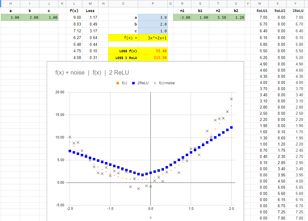
Quadratic Manual 2 ReLU
In this sheet you can try to find the best m1, b1, m2, b2 in order to make 2 ReLU fit the same (or other) quadratic equation.
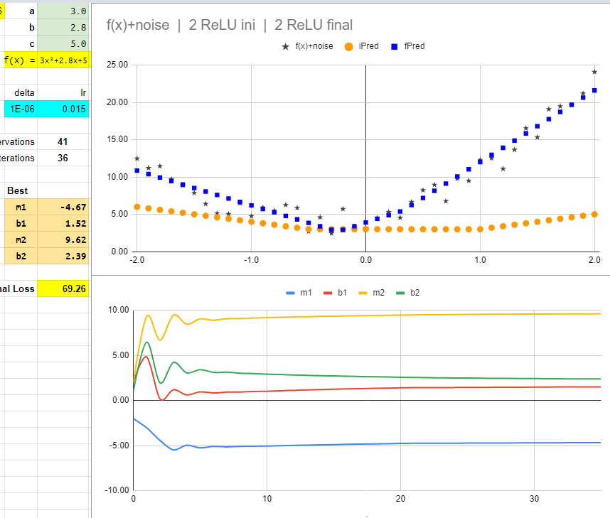
Quadratic 2ReLU GD
Gradient descent is again applied to find the best m1, b1, m2, b2.
Begining with base parameters as -2.00, 2.00, 2.00, 1.00. And a learning rate of 0.015.
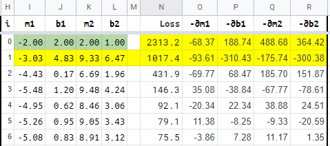
After 36 iterations (copying and pasting), we end up with a loss of 69.26 (For the points generated with noise, the fundamental 3x²+2x+1 has a loss of 55.48).
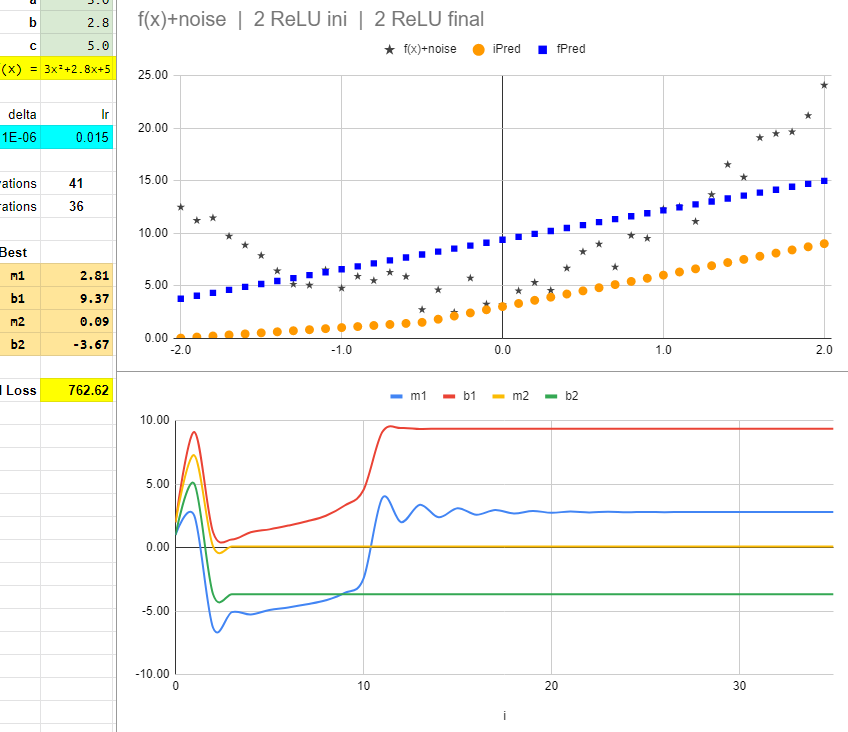
With this model iterations are very sensitive to the changes in the learning rate or in the first values we choose. For example, if we change the initial m1 from -2.00 to 1.00 we get a not so good result:
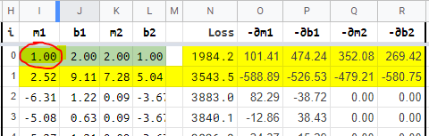
The model stabilizes as a full straight line with a loss of 762.62.
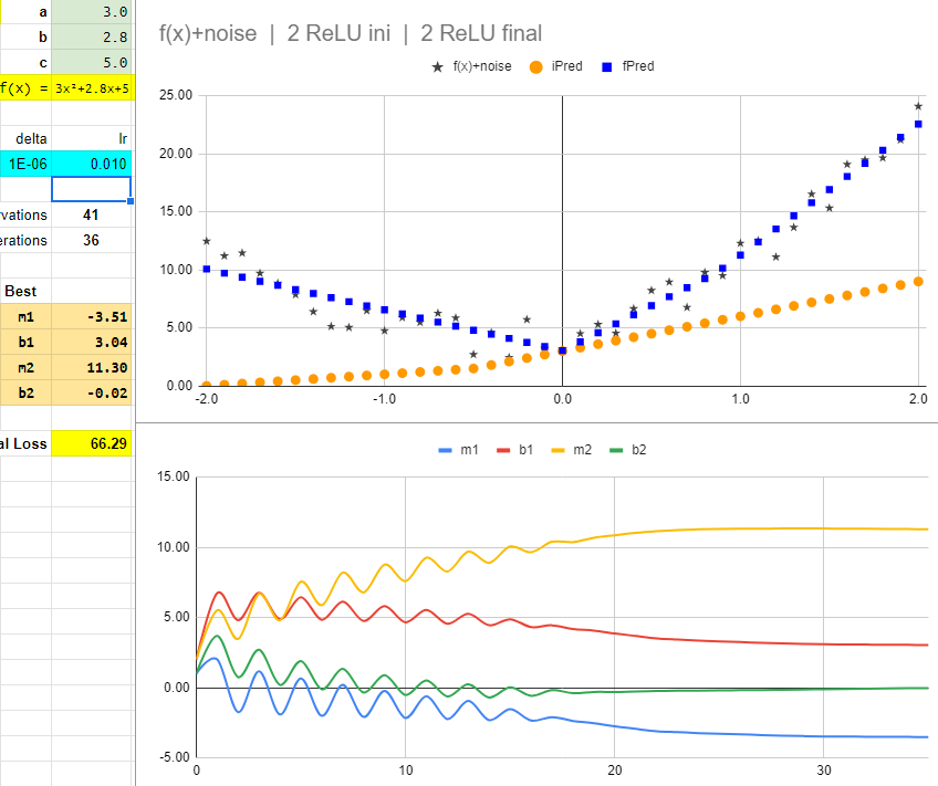
But if we now change the learning rate from 0.015 to 0.010, the parameters undulates a little, but then converge to a loss of 66.29.
And you can start trying learning rates of 0.01, 0.012, 0.013 and find the minimum loss (with all else equal).
You can also try more iterations by copy and pasting butween H and R columns.
Titanic 2ReLU [iter]
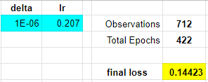
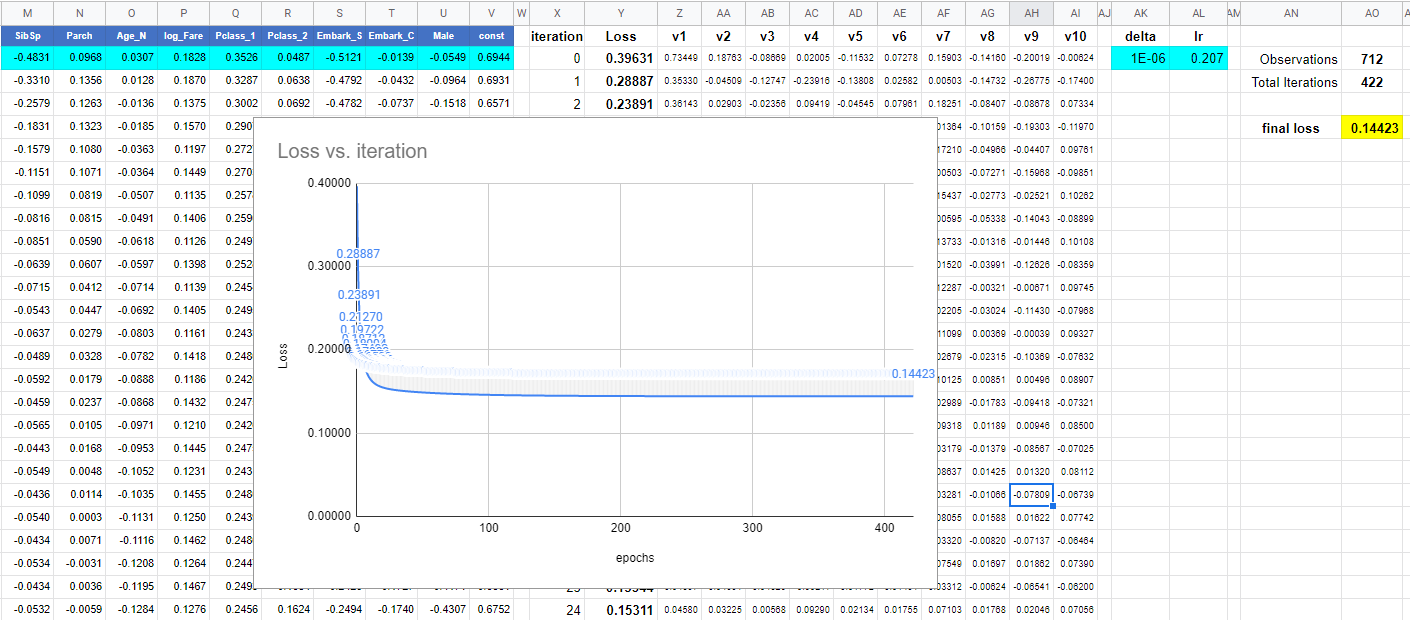
Here are two linear regressions, each with its own set of m1, m2, …, m9 and b1 parameters. Each iteration requires Google Sheets to calculate 20 derivatives. So changing some parameter or learning rate would need 20 derivatives for each iteration in the sheet. It takes about 1 minute for the 250 iterations that are defined in the sheet to update.
The model results and convergence gets very sensitive to the 20 different initial parameters an learning rates.
First try
With the following initial parameters:
| m11 |
m12 |
m13 |
m14 |
m15 |
m16 |
m17 |
m18 |
m19 |
b1 |
|
m21 |
m22 |
m23 |
m24 |
m25 |
m26 |
m27 |
m28 |
m29 |
b2 |
| -0.48 |
0.10 |
0.03 |
0.18 |
0.35 |
0.05 |
-0.51 |
-0.01 |
-0.05 |
0.69 |
|
0.00 |
-0.10 |
-0.10 |
0.20 |
0.40 |
-0.50 |
1.00 |
0.00 |
-1.00 |
0.00 |
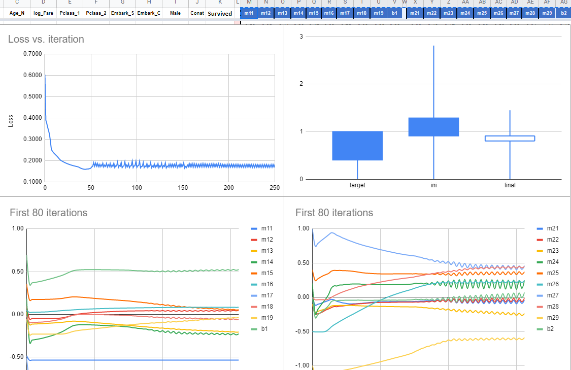
And a “big” learning rate of 0.35, we can see the process gets unstable after iteration 50.
Second try
By only changing the learning rate to 0.19, the model converge and the “distribution” of final predictions looks more like the target distribution than the initial predictions:
Titanic 2ReLU [iter] Solver
The initial aproximations used in this sheet are copied from predictions made with Excel Solver. So here the model is starting with very good parameters. So the iterations are to fine tune the already good parameters.
But what if we start the tuning with a leraning rate of 0.19?
First try
As we can see, a very musical model, but not so good in converging.
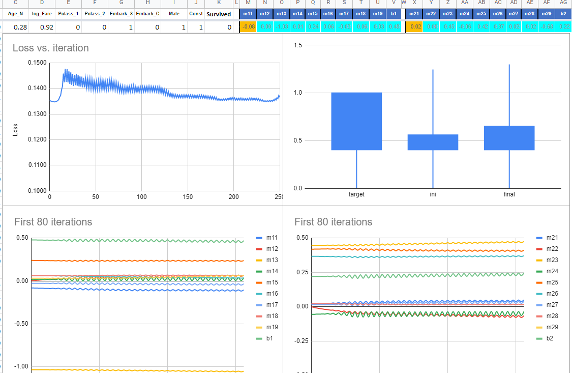
Second try
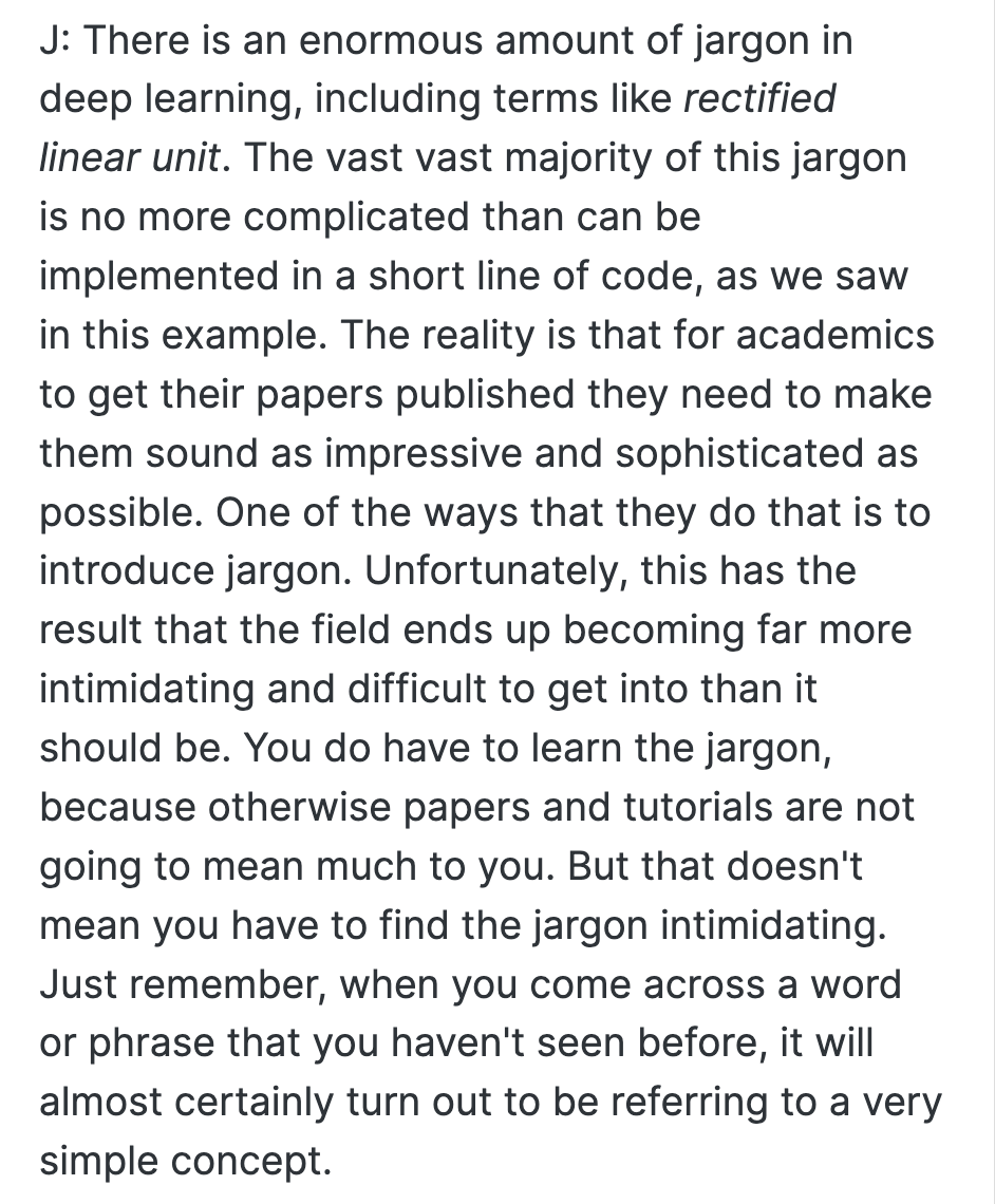
With a learning rate of 0.11 and 250 iterations, we get a small reduction in the loss from 0.13530 to 0.13363.
The two parameters that changed the most in the 250 iterations were m12 and m22…
Conclusions
- Maybe not the best way to practice the concepts involved, but hopefully useful in some other ways.
- Would be fun to try some of the Sheets ideas or plots in python.
- Making this Sheet definitively gave me a good insight about gradient descent and ReLU.
- Tweaking the parameters in Sheets was a great way to see how changing a hyperparameter like the learning rate or the initial estimations of a parameter can affect the fitting process and its convergence.