Live coding 16

I read somewhere that if you don’t have non linearities in between, then it’s as if you’re just doing logistic regression. I wish I remembered which lecture it was.

1 Like

Thanks to @fmussari for sharing the colab for searching youtube! I found the following by using the colab.

Hi Mike, here is Jeremy answering the question on Affine function in which he talked about:

  • What is an Affine function (linear function)? What does it do? (matrix multiplication and sum up)
  • What does it mean by adding one Affine function on top of another? (still another linear function)
  • What does it do by putting a non-linear activation (ReLU) in between Affine functions? (essentially building a neuralnet)

More to explore?

There are some good papers or posts we should read on ReLU or non-linear function in general to just have a one-step further understanding of the magic of non-linear function to neuralnet?

2 Likes

Like @Moody pointed out in previous posts, Jeremy also said the same in the fastbook that stacking 2 neurons (or linear functions) without non-linear activation in between “will just be the same as one linear” model.

However, as I showed the excel experiment in previous posts, a 2-linear function stacking on each other is a model much worse than (not the same as) a single linear model. How should I understand it? Is it something wrong with my experiment? @jeremy

Let me briefly describe the experiment: based on Jeremy’s 1-neuron model (1 linear layer model) with 2 weights a and b trying to find y=2x+30, I built a 2-neuron model (2 linear layer model) with 4 weights a, b, c and d to do the same. Both models share the exact same dataset, same learning rate, same initial weights (all set to 1). Both use the numerical derivative formula to calculate derivatives. you can check my numerical derivative formula here. You can run the experiment on the worksheet “basic SGD 2 neuron collapse” from this workbook.

1 Like

The main issue is that gradient descent doesn’t necessarily find the best answer. In high dimensions (e.g big neural nets) it generally gets pretty close, if you’ve got a good learning rate. But in low dimensions, it often doesn’t.

So experiments like this won’t tell you much about performance on real models, unfortunately.

5 Likes

Thank you Jeremy!

My understanding of what you said above is:
Among neural nets (non-linear functions added), in low dimensions, meaning among narrow and non-deep neural nets, SGD does not always find the best answer for the slightly bigger models; but in high dimensions, between large neural nets, SGD with good learning rate generally can help large models get closer to the optimal than smaller ones. ( This makes a lot of sense, and I’d like take this to be true)

And I assume when you mention ‘high and low dimensions’, you only refer to neural nets with nonlinearity (and there is no such thing as neural nets without nonlinearity, right?), correct?

Because in the book and in videos you are saying multiple linear functions on top of each other is just another single linear function with different weights. So, there is no high and low dimension difference between a single linear model and a model of multiple linear function on top of each other without nonlinearity.

S: Mathematically, we say the composition of two linear functions is another linear function. So, we can stack as many linear classifiers as we want on top of each other, and without nonlinear functions between them, it will just be the same as one linear classifier.

An intuitive expectation would be the mathematical similarity between a single linear function model and a model of multiple linear functions on top of each other should suggest the same or very similar on model performance.

To be more specific:

In the book and lectures you said stacking multiple linear functions together is really just “a single linear layer with a different set of parameters” e.g. a 2-linear functions model can be collapsed into y = acx + c*b+d. So, we would expect this collapsed linear model would perform the same or very similar as our y = ax + b if not better. But the experiment shows this collapsed linear model cannot even finish training a single epoch, not mentioning the terrible error.

So, Does it suggest from perspective of model performance the two models are not the same, even though mathematically they are the same?

Mathematically the trained model is the same. But the optimisation problem is different – with more parameters, there are more identical possible solutions, which is bad for SGD.

1 Like

Thanks a lot! This is very helpful!

Sarada has set a great example on how to visualize ReLU to enhance understanding. Here let’s try to do the same to Momentum.

What does Momentum look like

momentum = exponentially weighted moving average

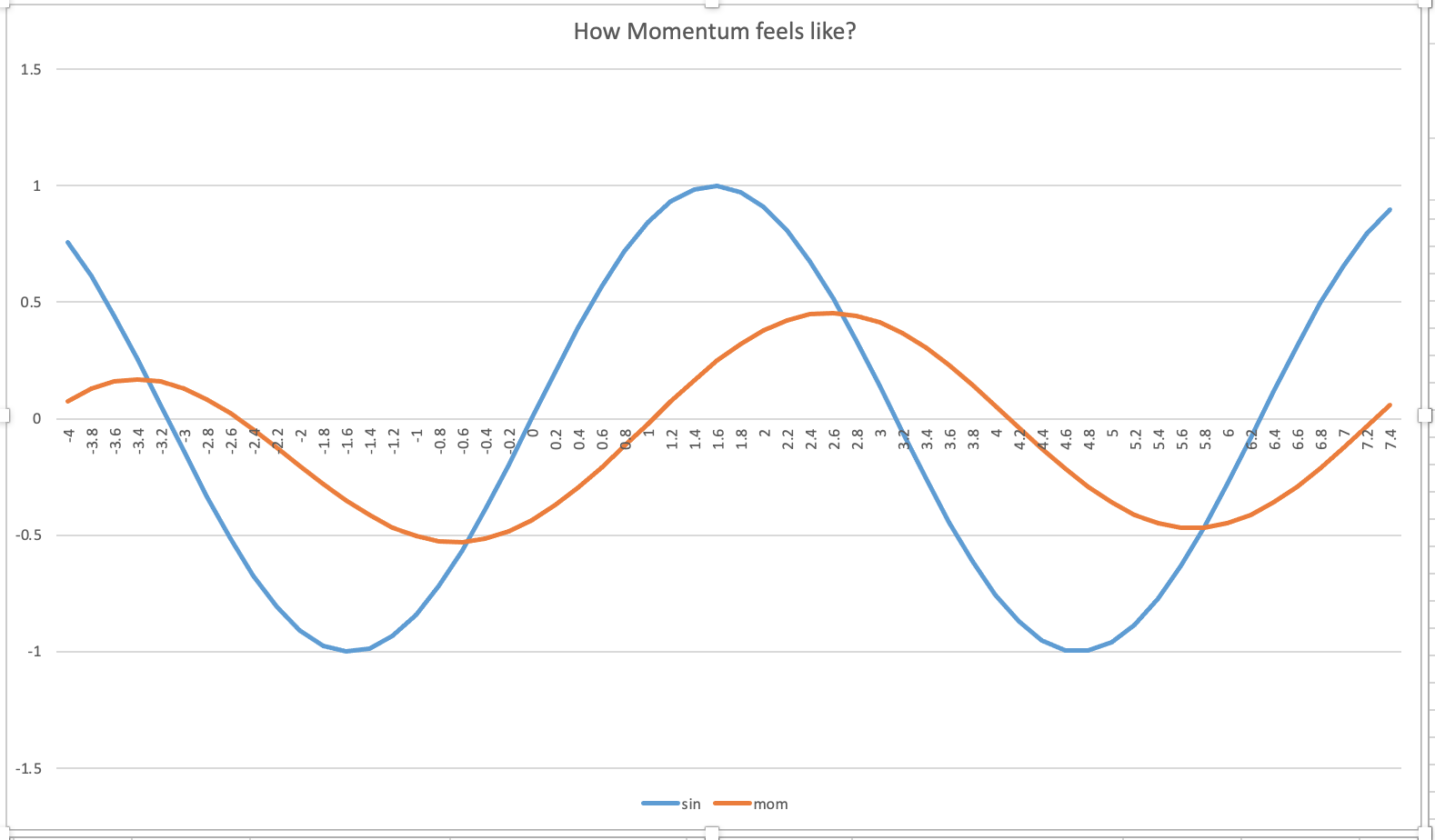
Basically, you can apply Momentum to a wiggly line. In the first example below we are using momentum to smooth y = sin(x) out. It smooths the line by give a large weight (in deep learning the convention is 90% on the previous momentum value and 10% weight to sin(x). so we have the momentum formula to be

mom(sin(x_t)) = 0.9*mom(sin(x_{t-1})) + 0.1*sin(x_t)

Why need momentum in deep learning?

We use SGD to update weights using derivatives. Derivatives like to swing between large positive and negative values. As a result, weight values swing too.

The intuition of momentum I suspect to be:
Weights jumping back and forth in big steps won’t bring them to the optimal efficiently. But if weights can keep their movement momentum, and gradually increase the steps, there should be higher chance of getting to the optimal.

First Example: Let’s visualize the momentum function

In this experiment we apply momentum formula to a sine function, and plot it to see how they look. Note: I set the first original momentum value to be 0

Can you get a feel about how momentum smooth things out or keep the momentum of previous state from the graph below?

Second Example: Let’s visualize momentum when applied on derivatives of weight

The derivatives of weights on each data point can be very wiggly. I have plotted the derivatives of weight d on our 2-neuron model. Their only difference is whether they use ReLU and Momentum or not. “no ReLU” is a derivative in the model without ReLU, “ReLU” means a derivative in the model with ReLU, “under mom” means a derivative in the model using ReLU and Momentum, “mom” means the momentum value in the model using ReLU and Momentum.

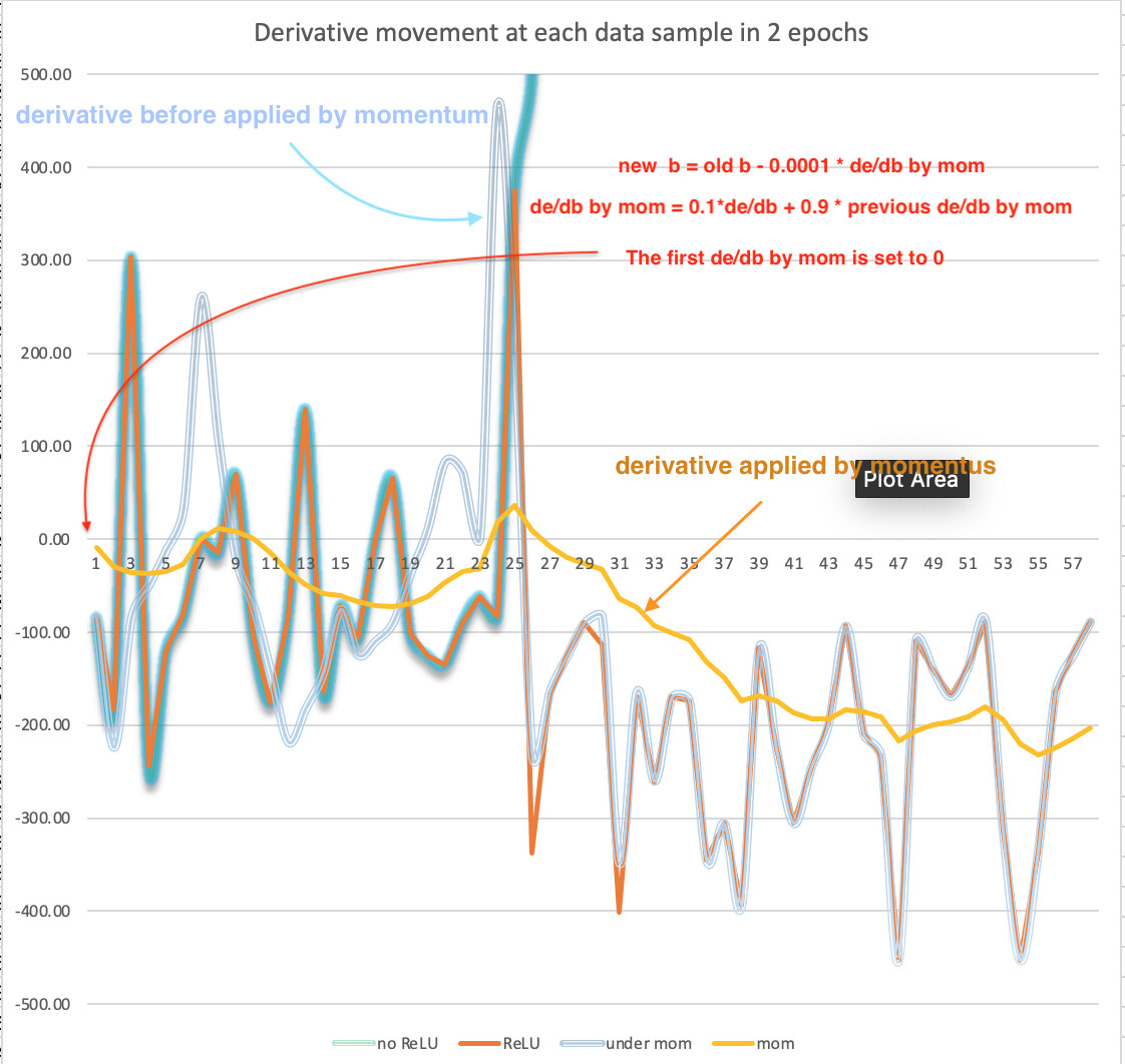
You can try out the spreadsheet above from here on the worksheet named “Plot momentum”

How Jeremy taught momentum? 2018, 2019

Jeremy explained the use of momentum in two use cases which I only came to get my head around them when I do this experiment today. (Please correct me if I am still not accurate in my understanding on them)

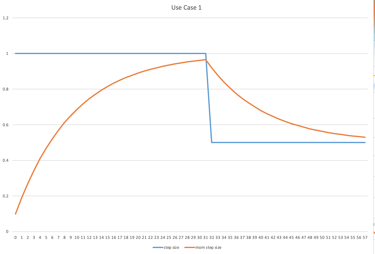
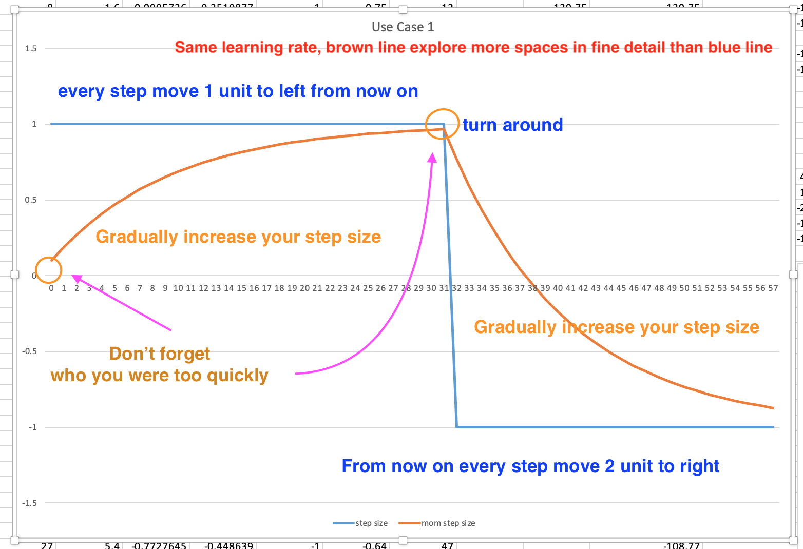
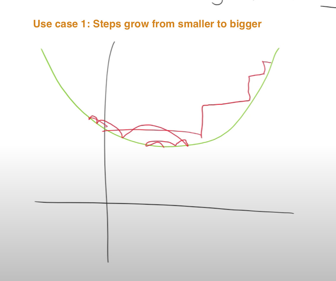
Use Case 1: when derivatives are not jumping big and back and forth

Momentum: remember where you were and don’t jump at a full change, only increase the change or step size gradually, so that you can explore more fine space having lower probability of stepping over the optimal (see the graph from the experiment). When your larger steps meet a derivative shows opposite direction with large value, then you are forced to turn around, still increase your steps gradually like above. (also see Jeremy’s drawing below)


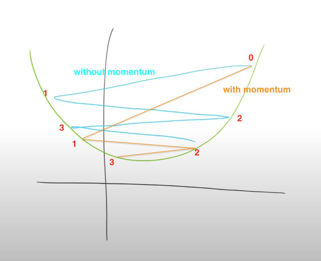
Use case 2: when derivatives are jumping in large steps and back and forth

when derivatives are jumping in large steps and back and forth, it is not very efficient in finding the optimal. But when derivatives do jump back and forth, momentum can keep them jump in smaller steps so that you are closer to the optimal than without momentum. ( see the graph illustration below)

Questions

There is something which is confusing when Jeremy talked about use case 1:

“If you are here and your learning rate is too small, if you keep doing the same steps, then if you also add in the step you took last time, and then your steps are getting bigger and bigger aren’t they? Until eventually they go too far …”

This quote sounds like “the same steps” are too smaller but after applied momentum, they will become bigger and bigger. But this interpretation can’t be right. According to our experiment below, if the same steps are always 1 and also greater than the initial momentum step 0, then the increasing momentum steps can never be bigger than 1. Then if sudden the same steps are changed to 0.5 and remain on this value onward, then the step value produced by momentum will decrease but is always greater than 0.5. (If I am wrong here, could anyone help me get this straight? thanks)

1 Like

Hi @Moody

When I am walking through the code for momentum in fastai source, I could not find the test for average_grad in the fastai folder. But I did find a test in the docs. Is there a test for average_grad in the fastai source?

If no, does it mean average_grad won’t get tested every time when the library is updated?


Well a sleep certainly helps :grin: I found it in nbs/12_optimizer.ipynb. I guess the problem is ctags won’t find average_grad in nbs folder and github does not search in jupyter notebooks files.

2 Likes

Hi Sarada, I am experimenting LAMBDA in excel to write an average_grad function from fastai’s average_grad. I have used both LAMBDA and LET in excel and the formula as you can imagine is very long. How can I write the long formula in excel nicely (without in a long line, which is unreadable) and even debug it along the way? Could you share some tips? Thanks!

=LAMBDA(p.grad.data, mom, dampening, grad_avg, LET(ini_grad, if(grad_avg="None", RANDARRAY(ROWS(p.grad.data), COLUMNS(p.grad.data),,,,False)*0, grad_avg), damp, if(dampening=FALSE, 1.0, 1-mom), p.grad.data*mom+grad_avg*damp))

I have reproduced average_grad and two of its tests (from fastai) in Excel without using LAMBDA and LET in this workbook. The notes in the cells of the spreadsheet give some hints how to use the spreadsheet. You can get a reminder of the average_grad and its tests by experiment them (fastai code) in the binder.

1 Like

I hope the below is self-explanatory.

Personally, I prefer Option 2. It is easier to debug during development. In businesses, essential models will be audited by internal or external parties. So readability is crucial.

Bonus point: Option 2 allows for keeping track of your parameters and the corresponding experimental results. Using visualisation, you can gain insight into what works or doesn’t.

I will check your workbook and binder later. I am having fun coding in APL. :star_struck:

Most importantly, you are practising what you learn. “Add oil”!!! (in Chinese) :star:

2 Likes

I would suggest looking into using VBA for creating user defined functions, in situations where a LAMBDA gets a big unwieldy.

3 Likes

Thank you Sarada, I got it. Now I have Gradually built up the Lambda from step by step directly based on the non-lambda version, which is readable and debuggable.

1 Like

Thank you Jeremy, when it gets really big unwieldy I may look into VBA. So far, the length of my lambda function seems manageable at the moment after I break it and implement it step by step.

1 Like

Eventually, yes, I think I will write those lambda function into VBA functions as once you built those lambda functions and start to use them, they provide no clues on how many parameters you should enter and what they mean, unlike custom functions created by VBA.

When I was writing this post to report I failed and gave up on getting VBA custom function work on descriptions of func and args, in order to write and reproduce the problem again I did a few more experiments and finally figured out why it didn’t work before or how I misused it.

Here is the code I use for creating docs for a dummy custom VBA function:


Function addNum(num1 As Double, num2 As Double) As Double

    addNum = num1 + num2

End Function

Sub doc_addNum()

Dim Arg(1 To 2) As String
Arg(1) = "number one"
Arg(2) = "number two"

    Application.MacroOptions Macro:="addNum", Description:="do it one last time to add two numbers with args", _
    ArgumentDescriptions:=Arg()
    
End Sub

Put it simply, to make docs (description for func and args) work, I just have to run this macro first which I had wrongly assumed it would run whenever the function is run, and spent too much time worrying about where is wrong with my codes and Excel settings.

Although the docs is working now, I do have an error when running the macro code.


Do you know what’s wrong with this line of code? @Moody

Hi @Daniel , VBA and Marco did not play nice with Document Management System which led to in breach of company policies. So, I don’t have much experience with them.

Since you start coding in VBA, why not do it in Python??? The learning curves will be similar. But, you can do more with Python. Pandas and Matplotlib can do simple charts without too much effort. Lots of online examples are available. The charting can be part of the wider experiment in Jupyter Notebook as well. So, everything will be kept in one place.

At some stage, Excel will limit what you can do. Although I inspired you to use it, as soon as you gain enough insight to understand the concepts. It is high time to move on to learn Python. :man_student:

2 Likes

You are very right about it! I have been thinking about how to draw a line between Excel and Jupyter notebook with python, and make the most out of the two.

As you said, gaining insight to understand concepts is where Excel’s specialty lies. As Jeremy demonstrated in his spreadsheets, get everything out in front of you and how they play together can illuminate the problem, especially when there are interesting connections (e.g., input image pixels and filters and activations) between them to be visualized, I guess this is what I will focus on using Excel, so sticking to Jeremy’s spreadsheets and think of how to make the most out of them. Everything else could be in Jupyter notebook and Python.

Currently I use pdb to experiment and understand 12_optimization notebook of fastai library, and before this I was thinking using Excel to illuminate on the difference between l2_reg and weight_decay. But now, maybe it is more convenient to just experiment and visualize in python. I will give it a try later.

2 Likes

Here is how I construct average_grad in Excel using LAMBDA and LET step by step based on the version without them.


Here is the spreadsheet

1 Like

Verify a warning message of fastai library through experiment in Excel

I have implemented weight_decay, l2_reg plus previously momentum_step and average_grad in Excel to prove a warning message (see below) from fastai doc

Here is the graph from the Excel experiment to prove the warning message above. The plot on the right shows that [weight_decay, momentum_step] is visually different from [l2_reg, momentum_step].

However, as you said this could be done in jupyter notebook. I suspect the calculation process could be less messy in jupyter notebook with python. Also using fastai in Jupyter notebook directly can verify the experiment of Excel.

Next steps:
I will try to make the experiment in Excel tidier and try to make it equivalent to fastai in python as much as possible. As for verification, I can simply compare the data generated by Excel and Jupyter notebook .