Deep Learning na Unb (Brasília) - Parte 1 - Lição 5

[ <<< Lição 4 | Lição 6 >>> ]

Lesson 5 - Foundations of Neural Networks (20/11/2019 - UnB - Brasília)

Este tópico permite que os membros do Grupo de IA da UnB (Brasília) estudem coletivamente (em reuniões presenciais e on-line) a lição 5 (parte 1) do curso fastai , mas de um jeito aberto para ajudar também pelas questões, respostas e pelos recursos publicados todos os leitores em português interessados em DL.

Lesson resources

Other resources

2 Likes

Ementa (20/11/2019 - UnB - Brasília)

  1. [ 20mn ] O que aconteceu online desde a aula precedente
  2. [ 20mn ] Lista dos projetos
  3. [ 15mn ] Organização da conferência de dezembro (data, horário, lugar, responsável geral, responsável da logística, responsável da comunicação, mentor dos projetos = Pierre)
  4. [ 10mn ] Pontos-chave da turma anterior
  5. [ 30mn ] lição 5 (veja “Videos timeline”)
  6. [ 1h25mn ] Oficinas práticas
    • Imagens (Pierre)
    • NLP (Thiago)
  7. [ 0mn ] Fotos da aula :slight_smile:

Videos timeline

  • Review of last week + parameters or weights/activations + backpropagation [3:32]
  • Fine tuning [8:45]
  • Freezing layers + Unfreezing and Using Discriminative Learning Rates [13:00]
  • Affine Function (matrix multiplication, linear function) [20:24]
  • Embedding [22:51]
  • Embedding once over + latent factors/features [27:57]
  • Bias [33:08]
  • Jeremy’s tricks for getting better results [43:18]
  • Interpreting bias [49:29]
  • Interpreting Weights + pca [54:27]
  • collab_learner + nn.Module + forward() [1:00:43]
  • Embeddings are amazing [1:07:03]
  • Regularization: Weight Decay [1:12:09]
  • Going back to Lesson2 SGD notebook [1:19:16]
  • MNIST SGD [1:23:59]
  • MNIST neural network [1:40:33]
  • Adam [1:43:56]
  • Momentum [1:48:40]
  • RMSProp [1:53:30]
  • Adam [1:55:44]
  • Fit one cycle [2:00:02]
  • Back to Tabular + Cross-Entropy Loss function + Regularization (weight decay, BatchNorm, dropout, Data Augmentation) [2:03:15]

Recursos

Exercícios até a próxima aula

  • Publique em seu blog sua compreensão do que é:
    • Embeddings
    • Affine function (matrix multiplication, linear function) and Bias
    • Transfer Learning and fine-tuning (freeze, unfreeze, Discriminative Learning rate)
    • Adaptative Learning rate (momentum, RMSProp, Adam, learn.fit_one_cycle())
    • Regularization (weight decay)
    • Loss function (MSE, CrossEntropyLoss())
  • Execute novamente seus primeiros notebooks sobre classificação de imagens com esses novos truques e tente melhorar o conteúdo de seus modelos (atualize as postagens relacionadas)
1 Like

How do we do discriminative learning rates in fastai?

Source: Unfreezing and Using Discriminative Learning Rates from lesson5.md

Anywhere you can put a learning rate in fastai such as with the fit function. The first thing you put in is the number of epochs and then the second thing you put in is learning rate (the same if you use fit_one_cycle ). The learning rate, you can put a number of things there:

  • You can put a single number (e.g. 1e-3 ): Every layer gets the same learning rate. So you’re not using discriminative learning rates.
  • You can write a slice. So you can write slice with a single number (e.g. slice(1e-3) ): The final layers get a learning rate of whatever you wrote down ( 1e-3 ), and then all the other layers get the same learning rate which is that divided by 3. So all of the other layers will be 1e-3/3 . The last layers will be 1e-3 .
  • You can write slice with two numbers (e.g. slice(1e-5, 1e-3) ). The final layers (these randomly added layers) will still be again 1e-3 . The first layers will get 1e-5 , and the other layers will get learning rates that are equally spread between those two - so multiplicatively equal. If there were three layers, there would be 1e-5 , 1e-4 , 1e-3 , so equal multiples each time.

One slight tweak - to make things a little bit simpler to manage, we don’t actually give a different learning rate to every layer. We give a different learning rate to every “layer group” which is just we decided to put the groups together for you. Specifically what we do is, the randomly added extra layers we call those one layer group. This is by default. You can modify it. Then all the rest, we split in half into two layer groups.

By default (at least with a CNN), you’ll get three layer groups. If you say slice(1e-5, 1e-3) , you will get 1e-5 learning rate for the first layer group, 1e-4 for the second, 1e-3 for the third. So now if you go back and look at the way that we’re training, hopefully you’ll see that this makes a lot of sense.

This divided by three thing, it’s a little weird and we won’t talk about why that is until part two of the course. It’s a specific quirk around batch normalization. So we can discuss that in the advanced topic if anybody’s interested.

What means embedding?

Source: Embedding once over from lesson5.md

You might have heard this word “embedding” all over the places as if it’s some magic advanced mathy thing, but embedding means look something up in an array. But it’s interesting to know that looking something up in an array is mathematically identical to doing a matrix product by a one hot encoded matrix. And therefore, an embedding fits very nicely in our standard model of our neural networks work.

Now suddenly it’s as if we have another whole kind of layer. It’s a kind of layer where we get to look things up in an array. But we actually didn’t do anything special. We just added this computational shortcut - this thing called an embedding which is simply a fast memory efficient way of multiplying by hot encoded matrix.

So this is really important. Because when you hear people say embedding, you need to replace it in your head with “an array lookup” which we know is mathematically identical to matrix multiply by a one hot encoded matrix.

Here’s the thing though, it has kind of interesting semantics. Because when you do multiply something by a one hot encoded matrix, you get this nice feature where the rows of your weight matrix, the values only appear (for row number one, for example) where you get user ID number one in your inputs. So in other words you kind of end up with this weight matrix where certain rows of weights correspond to certain values of your input. And that’s pretty interesting. It’s particularly interesting here because (going back to a kind of most convenient way to look at this) because the only way that we can calculate an output activation is by doing a dot product of these two input vectors. That means that they kind of have to correspond with each other. There has to be some way of saying if this number for a user is high and this number for a movie is high, then the user will like the movie. So the only way that can possibly make sense is if these numbers represent features of personal taste and corresponding features of movies . For example, the movie has John Travolta in it and user ID likes John Travolta, then you’ll like this movie.

We’re not actually deciding the rows mean anything. We’re not doing anything to make the rows mean anything. But the only way that this gradient descent could possibly come up with a good answer is if it figures out what the aspects of movie taste are and the corresponding features of movies are. So those underlying kind of features that appear that are called latent factors or latent features . They’re these hidden things that were there all along, and once we train this neural net, they suddenly appear.

What is bias?

Source: Bias from lesson5.md

Now here’s the problem. No one’s going to like Battlefield Earth. It’s not a good movie even though it has John Travolta in it. So how are we going to deal with that? Because there’s this feature called I like John Travolta movies, and this feature called this movie has John Travolta, and so this is now like you’re gonna like the movie. But we need to save some way to say “unless it’s Battlefield Earth” or “you’re a Scientologist” - either one. So how do we do that? We need to add in bias .

Here is the same thing again, the same construct, same shape of everything. But this time you’ve got an extra row. So now this is not just the matrix product of that and that, but I’m also adding on this number and this number. Which means, now each movie can have an overall “this is a great movie” versus “this isn’t a great movie” and every user can have an overall “this user rates movies highly” or “this user doesn’t rate movies highly” - that’s called the bias. So this is hopefully going to look very familiar. This is the same usual linear model concept or linear layer concept from a neural net that you have a matrix product and a bias.

And remember from lesson 2 SGD notebook, you never actually need a bias. You could always just add a column of ones to your input data and then that gives you bias for free, but that’s pretty inefficient. So in practice, all neural networks library explicitly have a concept of bias. We don’t actually add the column of ones.

What is a PyTorch layers and models?

Source: collab_learner from lesson5.md

in PyTorch, to remind you, all PyTorch layers and models are nn.Module 's. They are things that, once you create them, look exactly like a function. You call them with parentheses and you pass them arguments. But they’re not functions. They don’t even have __call__ . Normally in Python, to make something look like a function, you have to give it a method called dunder call. Remember that means __call__ , which doesn’t exist here. The reason is that PyTorch actually expects you to have something called forward and that’s what PyTorch will call for you when you call it like a function.

Regularization: Weight Decay [1:12:09]

Source: Regularization: Weight Decay from lesson5.md

We were trying to make sure we understood what every line of code did in this some pretty good collab learner model we built. The one piece missing is this wd piece, and wd stands for weight decay. So what is weight decay? Weight decay is a type of regularization. What is regularization?

Let’s start by going back to this nice little chart that Andrew Ng did in his terrific machine learning course where he plotted some data and then showed a few different lines through it. This one here, because Andrew’s at Stanford he has to use Greek letters. We can say this is but if you want to go there is a line. It’s a line even if it’s got a Greek letters. Here’s a second-degree polynomial - bit of curve, and here’s a high degree polynomial which is curvy as anything.

So models with more parameters tend to look more like this. In traditional statistics, we say “let’s use less parameters” because we don’t want it to look like this. Because if it looks like this, then the predictions far left and far right, they’re going to be all wrong. It’s not going to generalize well. We’re overfitting. So we avoid overfitting by using less parameters. So if any of you are unlucky enough to have been brainwashed by a background in statistics or psychology or econometrics or any of these kinds of courses, you’re gonna have to unlearn the idea that you need less parameters. Because what you instead need to realize is you were fed this lie that you need less parameters because it’s a convenient fiction for the real truth which is you don’t want your function to be too complex. Having less parameters is one way of making it less complex. But what if you had a thousand parameters and 999 of those parameters were 1e-9? What if they were 0? If they were 0, they’re not really there. Or if they were 1e-9, they’re hardly there. So why can’t I have lots of parameters if lots of them are really small? And the answer is you can. So this thing of counting the number of parameters is how we limit complexity is actually extremely limiting. It’s a fiction that really has a lot of problems. So if in your head complexity is scored by how many parameters you have, you’re doing it all wrong. Score it properly.

So why do we care? Why would I want to use more parameters? Because more parameters means more nonlinearities, more interactions, more curvy bits. And real life is full of curvy bits. Real life does not look like a straight line. But we don’t want them to be more curvy than necessary or more interacting than necessary. Therefore let’s use lots of parameters and then penalize complexity. So one way to penalize complexity (as I kind of suggested before) is let’s sum up the value of your parameters. Now that doesn’t quite work because some parameters are positive and some are negative. So what if we sum up the square of the parameters, and that’s actually a really good idea.

Let’s actually create a model, and in the loss function we’re going to add the sum of the square of the parameters. Now here’s a problem with that though. Maybe that number is way too big, and it’s so big that the best loss is to set all of the parameters to zero. That would be no good. So we want to make sure that doesn’t happen, so therefore let’s not just add the sum of the squares of the parameters to the model but let’s multiply that by some number that we choose. That number that we choose in fastai is called wd . That’s what we are going to do. We are going take our loss function and we’re going to add to it the sum of the squares of parameters multiplied by some number wd .

What should that number be? Generally, it should be 0.1. People with fancy machine learning PhDs are extremely skeptical and dismissive of any claims that a learning rate can be 3e-3 most of the time or a weight decay can be 0.1 most of the time. But here’s the thing - we’ve done a lot of experiments on a lot of datasets, and we’ve had a lot of trouble finding anywhere a weight decay of 0.1 isn’t great. However we don’t make that the default. We actually make the default 0.01. Why? Because in those rare occasions where you have too much weight decay, no matter how much you train it just never quite fits well enough. Where else if you have too little weight decay, you can still train well. You’ll just start to overfit, so you just have to stop a little bit early.

Function called update which calculated our predictions. That’s our weight make matrix multiply:

Source: SGD from lesson5.md

What’s our loss? Our loss is some function of our independent variables X and our weights (). In our case, we’re using mean squared error, for example, and it’s between our predictions and our actuals.

def update(x,y,lr):
    wd = 1e-5
    y_hat = model(x)
    # weight decay
    w2 = 0.
    for p in model.parameters(): w2 += (p**2).sum()
    # add to regular loss
    loss = loss_func(y_hat, y) + w2*wd
    loss.backward()
    with torch.no_grad():
        for p in model.parameters():
            p.sub_(lr * p.grad)
            p.grad.zero_()
    return loss.item()

Now you’re saying to PyTorch I want you to take these parameters and optimize them using SGD. So this now, rather than saying for p in parameters: p -= lr * p.grad , you just say opt.step() . It’s the same thing. It’s just less code and it does the same thing. But the reason it’s kind of particularly interesting is that now you can replace SGD with Adam for example and you can even add things like weight decay because there’s more stuff in these things for you. So that’s why we tend to use optim.blah . So behind the scenes, this is actually what we do in fastai.

L2 regularization and weight decay

Source: MNIST SGD from lesson5.md

That () is only interesting for training a neural net because it appears here (). Because we take the gradient of it. That’s the thing that actually updates the weights. So actually the only thing interesting about is its gradient. So we don’t do a lot of math here, but I think we can handle that. The gradient of this whole thing if you remember back to your high school math is equal to the gradient of each part taken separately and then add them together. So let’s just take the gradient of that () because we already know the gradient of this () is just whatever we had before. So what’s the gradient of ?

Let’s remove the sum and pretend there’s just one parameter. It doesn’t change the generality of it. So the gradient of - what’s the gradient of that with respect to ?

It’s just . So remember this () is our constant which in that little loop was 1e-5. And is our weights. We could replace with like without loss of generality, so let’s throw away the 2. So in other words, all weight decay does is it subtracts some constant times the weights every time we do a batch. That’s why it’s called weight decay.

  • When it’s in this form () where we add the square to the loss function, that’s called L2 regularization .
  • When it’s in this form () where we subtract times weights from the gradients, that’s called weight decay .

They are kind of mathematically identical. For everything we’ve seen so far, in fact they are mathematically identical. And we’ll see in a moment a place where they’re not - where things get interesting. So this is just a really important tool you now have in your toolbox. You can make giant neural networks and still avoid overfitting by adding more weight decay. Or you could use really small datasets with moderately large sized models and avoid overfitting with weight decay. It’s not magic. You might still find you don’t have enough data in which case you get to the point where you’re not overfitting by adding lots of weight decay and it’s just not training very well - that can happen. But at least this is something that you can now play around with.

Momentum

Source: Momentum from lesson5.md

The first thing we can do to speed it up is to use something called momentum. Here’s the exact same spreadsheet as the last worksheet. I’ve removed the finite differencing version of the derivatives because they’re not that useful, just the analytical ones here. de/db where I take the the derivative and I’m going to update by the derivative.

But what I do is I take the derivative and I multiply it by 0.1. And what I do is I look at the previous update and I multiply that by 0.9 and I add the two together. So in other words, the update that I do is not just based on the derivative but 1/10 of it is the derivative and 90% of it is just the same direction I went last time. This is called momentum. What it means is, remember how we thought about what might happen if you’re trying to find the minimum of this.

You were here and your learning rate was too small, and you just keep doing the same steps. Or if you keep doing the same steps, then if you also add in the step you took last time, and your steps are going to get bigger and bigger until eventually they go too far. But now, of course, your gradient is pointing the other direction to where your momentum is pointing. So you might just take a little step over here, and then you’ll start going small steps, bigger steps, bigger steps, small steps, bigger steps, like that. That’s kind of what momentum does.

If you’re going too far like this which is also slow all, then the average of your last few steps is actually somewhere between the two, isn’t it? So this is a really common idea - when you have something that says my step at time T equals some number (people often use alpha because gotta love these Greek letters) times the actual thing I want to do (in this case it’s the gradient) plus one minus alpha times whatever you had last time ():

This is called an exponentially weighted moving average . The reason why is that, if you think about it, these are going to multiply. So if is in here with and is in there with .

So in other words ends up being the actual thing I want () plus a weighted average of the last few time periods where the most recent ones are exponentially higher weighted. And this is going to keep popping up again and again. So that’s what momentum is. It says I want to go based on the current gradient plus the exponentially weighted moving average of my last few steps. So that’s useful. That’s called SGD with momentum, and we can do it by changing:

opt = optim.Adam(model.parameters(), lr)

to

opt = optim.SGD(model.parameters(), lr, momentum=0.9)

Momentum 0.9 is really common. It’s so common it’s always 0.9 (just about) four basic stuff. So that’s how you do SGD with momentum. And again I didn’t show you some simplified version, I showed you “the” version. That is SGD. Again you can write your own. Try it out. That would be a great assignment would be to take lesson 2 SGD and add momentum to it; or even the new notebook we’ve got MNIST, get rid of the optim. and write your own update function with momentum.

RMSProp

Source: RMSProp from lesson5.md

Then there’s a cool thing called RMSProp. One of the really cool things about RMSProp is that Geoffrey Hinton created it (a famous neural net guy). Everybody uses it. It’s like really popular and common. The correct citation for RMSProp is the Coursera online free MOOC. That’s where he first mentioned RMSProp so I love this thing that cool new things appear in MOOCs not a paper.

So RMSProp is very similar to momentum but this time we have an exponentially weighted moving average not of the gradient updates but of F8 squared - that’s the gradient squared. So what the gradient squared times 0.1 plus the previous value times 0.9. This is an exponentially weighted moving average of the gradient squared. So what’s this number going to mean? Well if my gradient is really small and consistently really small, this will be a small number. If my gradient is highly volatile, it’s going to be a big number. Or if it’s just really big all the time, it’ll be a big number.

Why is that interesting? Because when we do an update this time we say weight minus learning rate times gradient divided by the square root of this (shown as below).

So in other words, if our gradient is consistently very small and not volatile, let’s take bigger jumps. That’s kind of what we want, right? When we watched how the intercept moves so darn slowly, it’s like obviously you need to just try to go faster.

So if I now run this, after just 5 epochs, this is already up to 3. Where else, with the basic version after five epochs it’s still at 1.27. Remember, we have to get to 30.

Adam

Source: Adam from lesson5.md

So the obvious thing to do (and by obvious I mean only a couple of years ago did anybody actually figure this out) is do both. So that’s called Adam . So Adam is simply keep track of the exponentially weighted moving average of the gradient squared (RMSProp) and also keep track of the exponentially weighted moving average of my steps (momentum). And both divided by the exponentially weighted moving average of the squared terms and take 0.9 of a step in the same direction as last time. So it’s momentum and RMSProp - that’s called Adam. And look at this - 5 steps, we’re at 25.

These optimizes, people call them dynamic learning rates. A lot of people have the misunderstanding that you don’t have to set a learning rate. Of course, you do. It’s just like trying to identify parameters that need to move faster or consistently go in the same direction. It doesn’t mean you don’t need learning rates. We still have a learning rate. In fact, if I run this again, it’s getting better but eventually it’s just moving around the same place. So you can see what’s happened is the learning rateis too high. So we could just drop it down and run it some more. Getting pretty close now, right?

Note: Adam, a method for efficient stochastic optimization that only requires first-order gradients with little memory requirement. The method computes individual adaptive learning rates for different parameters from estimates of first and second moments of the gradients; the name Adam is derived from adaptive moment estimation.

Fit one cycle

Source: Fit one cycle from lesson5.md

Now what does fit one cycle do? What does it really do? This is what it really does:

We’ve seen this chart on the left before. Just to remind you, this is plotting the learning rate per batch. Remember, Adam has a learning rate and we use Adam by default (or minor variation which we might try to talk about). So the learning rate starts really low and it increases about half the time, and then it decreases about half the time. Because at the very start, we don’t know where we are. So we’re in some part of function space, it’s just bumpy as all heck. So if you start jumping around, those bumps have big gradients and it will throw you into crazy parts of the space. So start slow. Then you’ll gradually move into parts of the weight space that is sensible. And as you get to the points where they’re sensible, you can increase the learning rate because the gradients are actually in the direction you want to go. Then as we’ve discussed a few times, as you get close to the final answer you need to anneal your learning rate to hone in on it.

But here’s the interesting thing - on the right is the momentum plot. Every time our learning rate is small, our momentum is high. Why is that? Because I do have a learning small learning rate, but you keep going in the same direction, you may as well go faster. But if you’re jumping really far, don’t like jump really far because it’s going to throw you off. Then as you get to the end again, you’re fine tuning in but actually if you keep going the same direction again and again, go faster. So this combination is called one cycle and it’s a simple thing but it’s astonishing. This can help you get what’s called super convergence that can let you train 10 times faster.

This was just last year’s paper. Some of you may have seen the interview with Leslie Smith that I did last week. An amazing guy, incredibly humble and also I should say somebody who is doing groundbreaking research well into his 60’s and all of these things are inspiring.

Cross-Entropy loss function

Source: Back to Tabular from lesson5.md

loss_func = nn.CrossEntropyLoss()

Cross-entropy loss is just another loss function. You already know one loss function which is mean squared error . That’s not a good loss function for us because in our case we have, for MNIST, 10 possible digits and we have 10 activations each with a probability of that digit. So we need something where predicting the right thing correctly and confidently should have very little loss; predicting the wrong thing confidently should have a lot of loss. So that’s what we want.

Here’s an example:

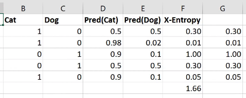
Here is cat versus dog one hot encoded. Here are my two activations for each one from some model that I built - probability cat, probability dog. The first row is not very confident of anything. The second row is very confident of being a cat and that’s right. The third row is very confident for being a cat and it’s wrong. So we want a loss that for the first row should be a moderate loss because not predicting anything confidently is not really what we want, so here’s 0.3. The second row is predicting the correct thing very confidently, so 0.01. The third row is predicting the wrong thing very confidently, so 1.0.

How do we do that? This is the cross entropy loss:

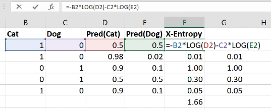
It is equal to whether it’s a cat multiplied by the log of the cat activation, negative that, minus is it a dog times the log of the dog activation. That’s it. So in other words, it’s the sum of all of your one hot encoded variables times all of your activations.

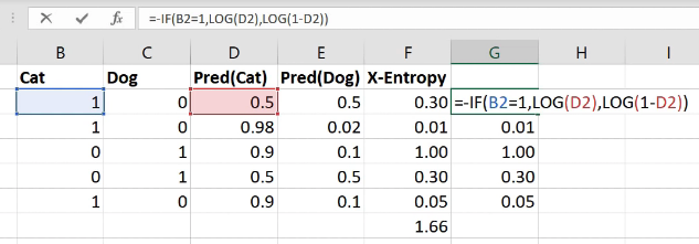
Interestingly these ones here (column G) - exactly the same numbers as the column F, but I’ve written it differently. I’ve written it with an if function because the zeros don’t actually add anything so actually it’s exactly the same as saying if it’s a cat, then take the log of cattiness and if it’s a dog (i.e. otherwise) take the log of one minus cattiness (in other words, the log of dogginess). So the sum of the one hot encoded times the activations is the same as an if function. If you think about it, because this is just a matrix multiply, it is the same as an index lookup (as we now know from our from our embedding discussion). So to do cross entropy, you can also just look up the log of the activation for the correct answer.

Now that’s only going to work if these rows add up to one. This is one reason that you can get screwy cross-entropy numbers is (that’s why I said you press the wrong button) if they don’t add up to 1 you’ve got a trouble. So how do you make sure that they add up to 1? You make sure they add up to 1 by using the correct activation function in your last layer. And the correct activation function to use for this is softmax . Softmax is an activation function where:

  • all of the activations add up to 1
  • all of the activations are greater than 0
  • all of the activations are less than 1

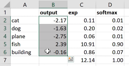
So that’s what we want. That’s what we need. How do you do that? Let’s say we were predicting one of five things: cat, dog, plane, fish, building, and these were the numbers that came out of our neural net for one set of predictions ( output ).

What if I did to the power of that? That’s one step in the right direction because to the power of something is always bigger than zero so there’s a bunch of numbers that are always bigger than zero. Here’s the sum of those numbers (12.14). Here is to the number divided by the sum of to the number:

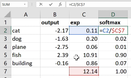
Now this number is always less than one because all of the things were positive so you can’t possibly have one of the pieces be bigger than 100% of its sum. And all of those things must add up to 1 because each one of them was just that percentage of the total. That’s it. So this thing softmax is equal to to the activation divided by the sum of to the activations. That’s called softmax.

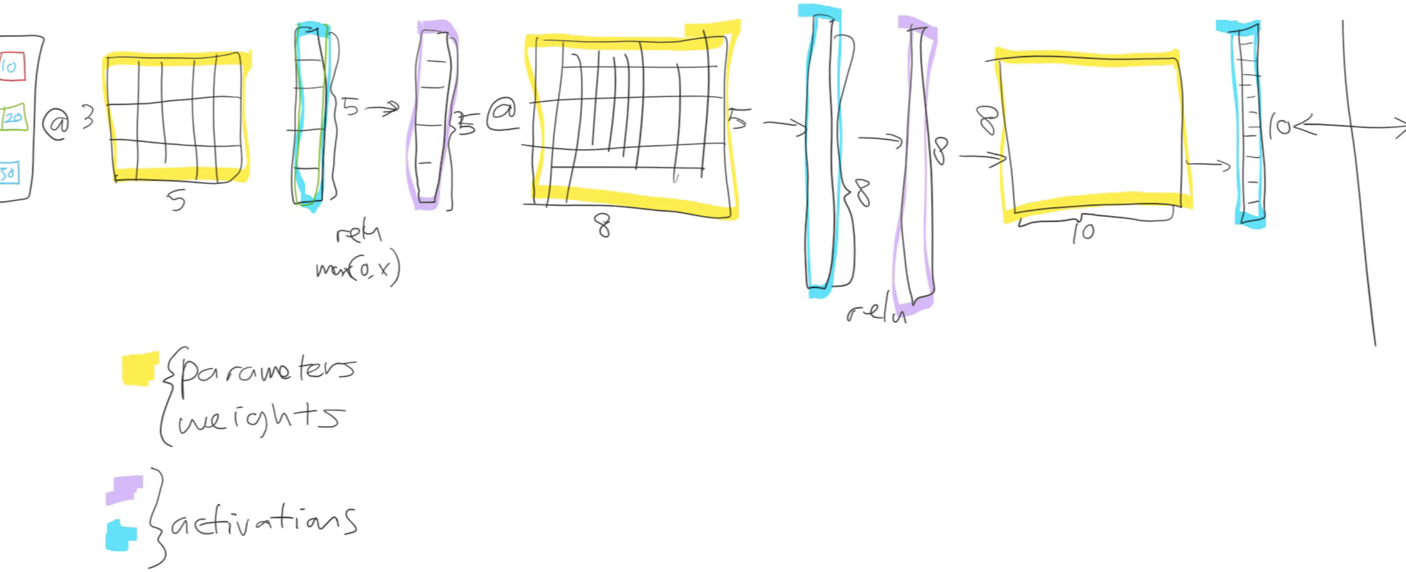
So when we’re doing single label multi-class classification, you generally want softmax as your activation function and you generally want cross-entropy as your loss. Because these things go together in such friendly ways, PyTorch will do them both for you. So you might have noticed that in this MNIST example, I never added a softmax here:

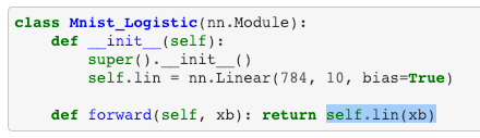
That’s because if you ask for cross entropy loss ( nn.CrossEntropyLoss ), it actually does the softmax inside the loss function. So it’s not really just cross entropy loss, it’s actually softmax then cross entropy loss.

So you’ve probably noticed this, but sometimes your predictions from your models will come out looking more like this:

Pretty big numbers with negatives in, rather than this (softmax column) - numbers between 0 to 1 that add up to 1. The reason would be that it’s a PyTorch model that doesn’t have a softmax in because we’re using cross entropy loss and so you might have to do the softmax for it.

Fastai is getting increasingly good at knowing when this is happening. Generally if you’re using a loss function that we recognize, when you get the predictions, we will try to add the softmax in there for you. But particularly if you’re using a custom loss function that might call nn.CrossEntropyLoss behind the scenes or something like that, you might find yourself with this situation.

Regularization

Source: Back to Tabular from lesson5.md

Next week when we finish off tabular which we’ll do in like the first 10 minutes, this is forward in tabular:

It basically goes through a bunch of embeddings. It’s going to call each one of those embeddings e and you can use it like a function, of course. So it’s going to pass each categorical variable to each embedding, it’s going to concatenate them together into a single matrix. It’s going to then call a bunch of layers which are basically a bunch of linear layers. And then it’s going to do our sigmoid trick.

There’s only two new things we’ll need to learn. One is dropout and the other is batch norm ( bn_cont ). These are two additional regularization strategies. BatchNorm does more than just regularization, but amongst other things it does regularization. And the basic ways you regularize your model are weight decay, batch norm, and dropout. Then you can also avoid overfitting using something called data augmentation.

So batch norm and dropout, we’re going to touch on at the start of next week. And we’re also going to look at data augmentation and then we’re also going to look at what convolutions are. And we’re going to learn some new computer vision architectures and some new computer vision applications.