📝 Deep Learning Lesson 5 Notes

We started with computer vision because it’s the most mature kind of out-of-the-box ready to use deep learning application. It’s something which if you’re not using deep learning you won’t be getting good results. So the difference you know hopefully between not doing lesson 1 versus doing lesson 1.

You’ve gained a new capability you didn’t have before and you kind of get to see a lot of the kind of tradecraft of training and effective neural network.

And so then we moved into NLP because the text is kind of another one which you really kind of can’t do really well without deep learning, generally speaking. It’s just got to the point where it works pretty well now.

In fact, the New York Times just featured an article about the latest advances in deep learning for text yesterday and talked quite a lot about the work that we’ve done in that area along with open AI, Google and Allen Institute of artificial intelligence.

NY Times Article - Finally, a Machine That Can Finish Your Sentence

We’ve kind of finished our application journey with tabular and collaborative filtering.
Tabular and collaborative filtering are the things that you can still do pretty well without deep learning so it’s not such a big step. It’s not a kind of whole new thing that you could do that you couldn’t use to do. And also because we’re going to try to get to a point where we understand pretty much every line of code and the
implementations of these things. Its implementation is much less intricate than vision and NLP.

So as we come down this other side of the journey which is like all the stuff we’ve just done, how does it actually work?

We will start from where we just ended which is collaborative filtering and then tabular data we’re going to be able to see what all those lines of code do by the end of today’s lesson. That’s our goal.

Particularly this lesson you should not expect to come away knowing how to solve applications you couldn’t do before but instead you should have a better understanding of how we’ve actually been solving the applications we’ve seen so far. We’re going to understand a lot more about regularization which is how we go about managing overfitting versus underfitting. Hopefully, you can use some of the tools from this lesson to go back to your previous projects and get a little bit more performance or handle models where previously maybe you felt like your data was not enough or maybe your underfitting and so forth.

It’s also going to lay the groundwork for understanding convolutional neural networks and recurrent neural networks that will do deep dives into in the next two lessons

And as we do that we’re also going to look at some new vision and NLP applications.

Components of deep Neural Network

[03:35]

Let’s start where we left off last week. Do you remember this picture?

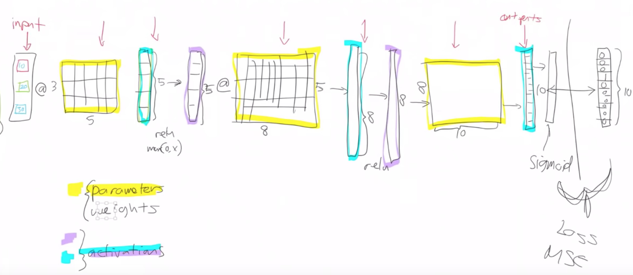
This picture describes what is a deep neural net look like. And we had various layers.

The first thing we pointed out is that there are only and exactly two types of layers -

Parameters - These are layers that contain parameters/weights, also called as linear layers which maintain state, For example, convolutions, linear.
Parameters are the things that your model learns, they’re the things that you use gradient descent to go.

parameter = parameter - learning_rate * parameter.grad

That’s our basic. That’s what we do.
And those parameters are used by multiplying them by input activations doing a matrix product.
The yellow things in the above diagram are our weight matrices, your weight tensors more generally.

Activations - These are layers that contain activations, also called as non-linear layers which are stateless. For example, ReLu or softmax.

We take some input activations or some layer activations and we multiply it by weight matrix to get a bunch of activations. Activations are numbers but they are calculated.
Jeremy says he keeps getting questions about where does that number come from? and he always answers it in the same way you tell me is it a parameter or is it an activation? because it’s one of those two things that’s where numbers come from.

I guess inputs a kind of a special activation so they’re not calculated they’re just there. Maybe that’s a special case.

Layers can be an input or a parameter or an activation.

Activations don’t only come out of matrix multiplications. They also come out of activation functions.

Element-wise function

The most important thing to remember about an activation function is that it’s an element-wise function. It’s a function that is applied to each element of the input, activations in turn and creates one activation for each input element. If it starts with a twenty long vector it creates a twenty long vector by looking at each one of those, in turn, doing one thing to it and spitting out the answer, so an element-wise function.

ReLu is the main one we’ve looked at and honestly, it doesn’t too much matter which you pick. so we don’t spend much time talking about activation functions because if you just use ReLu, you’ll get a pretty good answer all the time.

We also learned that this combination of matrix multiplications followed by ReLu’s stacked together has this amazing mathematical property called the Universal Approximation Theorem.
It says if you have big enough weight matrices and enough of them it can solve any arbitrarily complex mathematical function to any arbitrarily high level of accuracy. Assuming that you can train the parameters both in terms of time and data availability and so forth.

A visual proof that neural nets can compute any function

Backpropagation

[07:06]

This concept is which Jeremy finds more advanced. Computer scientists get really confused about how does it work?
It’s just you pass back the gradients and you update the weights with the learning rate. That piece where we take the loss function between the actual targets and the output of the final layer for the final activations. We calculate the gradients with respect to all of these parameters (yellow things) and then we update those weights by learning rate by subtracting learning rate times the gradient. This process of calculating those gradients and then subtracting like that is called backpropagation.
All this boils down to below formula.

weights = weights - weights.grad * learning rate

This is what we covered in lesson 4. We will come back to softmax and cross entropy today.

Fine-tuning

[08:45]

What happens when we take a resnet34 and we do transfer learning. What’s actually going on?

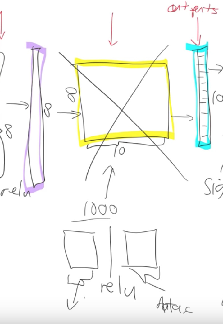
The first thing to notice is the resnet34 that we grabbed from Imagenet has a very specific weight matrix at the end. It’s a weight matrix that has 1000 columns. Because in Imagenet competition you have to figure out which one of these 1000 image categories this picture belongs to. That’s why in Imagenet this target vector is of length 1000. You’ve got to pick the probability that it’s which one of those 1000 things.

There are 2 reasons this weight matrix is no good to you when you’re doing transfer learning.

We probably don’t have a thousand categories. Jeremy was trying to do teddy bears, black bears or brown bears so he doesn’t want a thousand categories.
Even if we did have it exactly a 1000 categories they’re not the same 1000 categories that are in Imagenet.

So basically this whole weight matrix is a waste of time for us. What do we do we throw it away so when you go create_cnn() in fastai it deletes that. And instead, it puts in 2 new weight matrices in there for you with a ReLu in between.

So there are some defaults as to what size is the first one is but for the second one the size is as big as you need it to be. In your data bunch which you passed your learner from that, we know how many activations you need. If you’re doing classification it’s how many classes you have if you’re doing regression then how many numbers you’re trying to predict. Remember that in your if your data bunch is called data then that’ll be called

data.c

Fastai library will add for you this weight matrix of size data.c by however much was in the previous layer.

Visualizing and Understanding Convolutional Networks - Zeiler and Fergus Paper

[11:38]

Now we need to train those 2 weight matrices. Weight matrices are always full of random numbers if they’re new and these ones we’ve grabbed them and thrown them in there so we need to train them but the other layers are not new, they are good at something right and what are they good at?

Remember this paper Visualizing and Understanding Convolutional Networks from Zeiler and Fergus.

Below are some examples of visualizations of some filters or weight matrices and some examples of what they found.

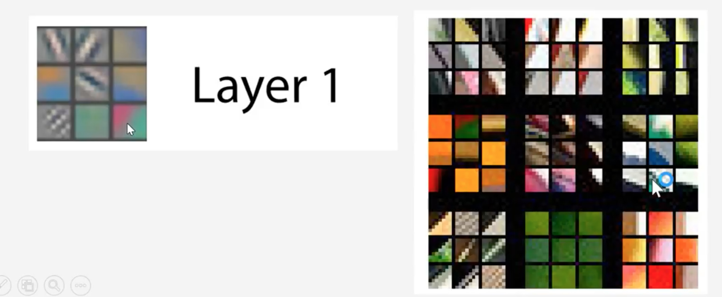
In layer 1, part of weight matrices was good at finding diagonal edges in different directions.

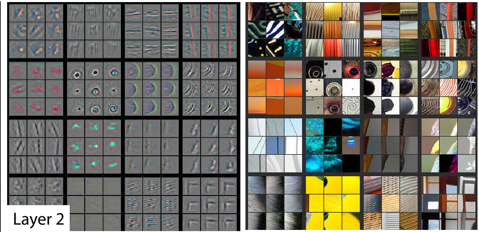
In layer 2, some of the filters were good at spotting corners in the bottom right corner.

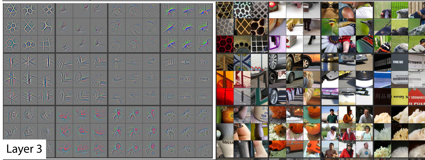
In layer 3, one of the filters found repeating patterns or round orange things or fluffy or floral textures.

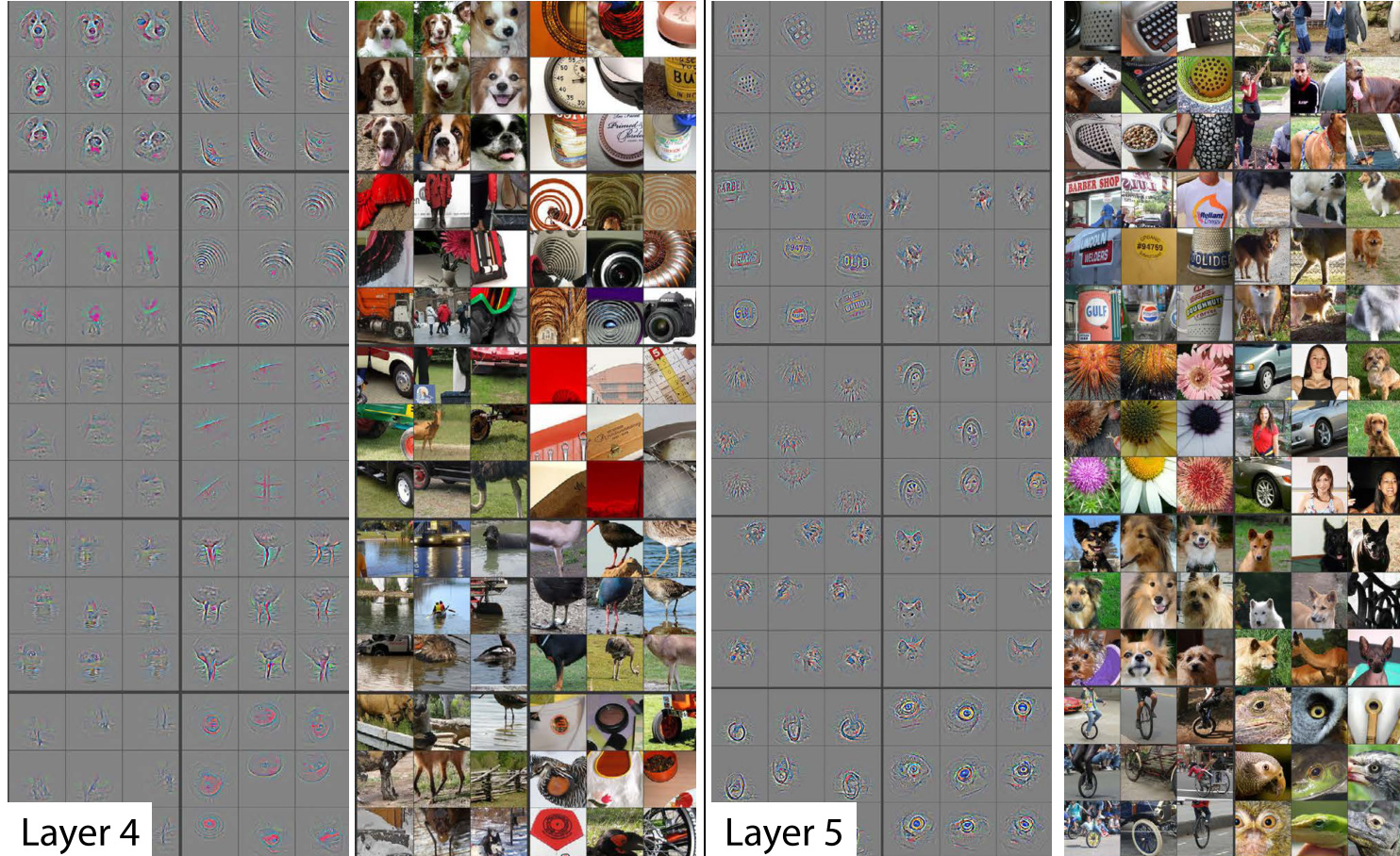
As we go deeper, they’re becoming more sophisticated but also more specific.
By layer 5, It could find bird eyeballs or dog faces.

Check lesson1 notes for more on this paper.

For example, if you’re wanting to transfer and learn to something for histopathology slides there’s probably going to be no eyeballs in that. So the later layers are no good to you but there will certainly be some repeating patterns or some diagonal edges. The earlier you grow in the model the more likely it is that you want those weights to stay as they are.

Freezing layers - (Not updating weights)
53%20AM1382×944 161 KB

[13:00]

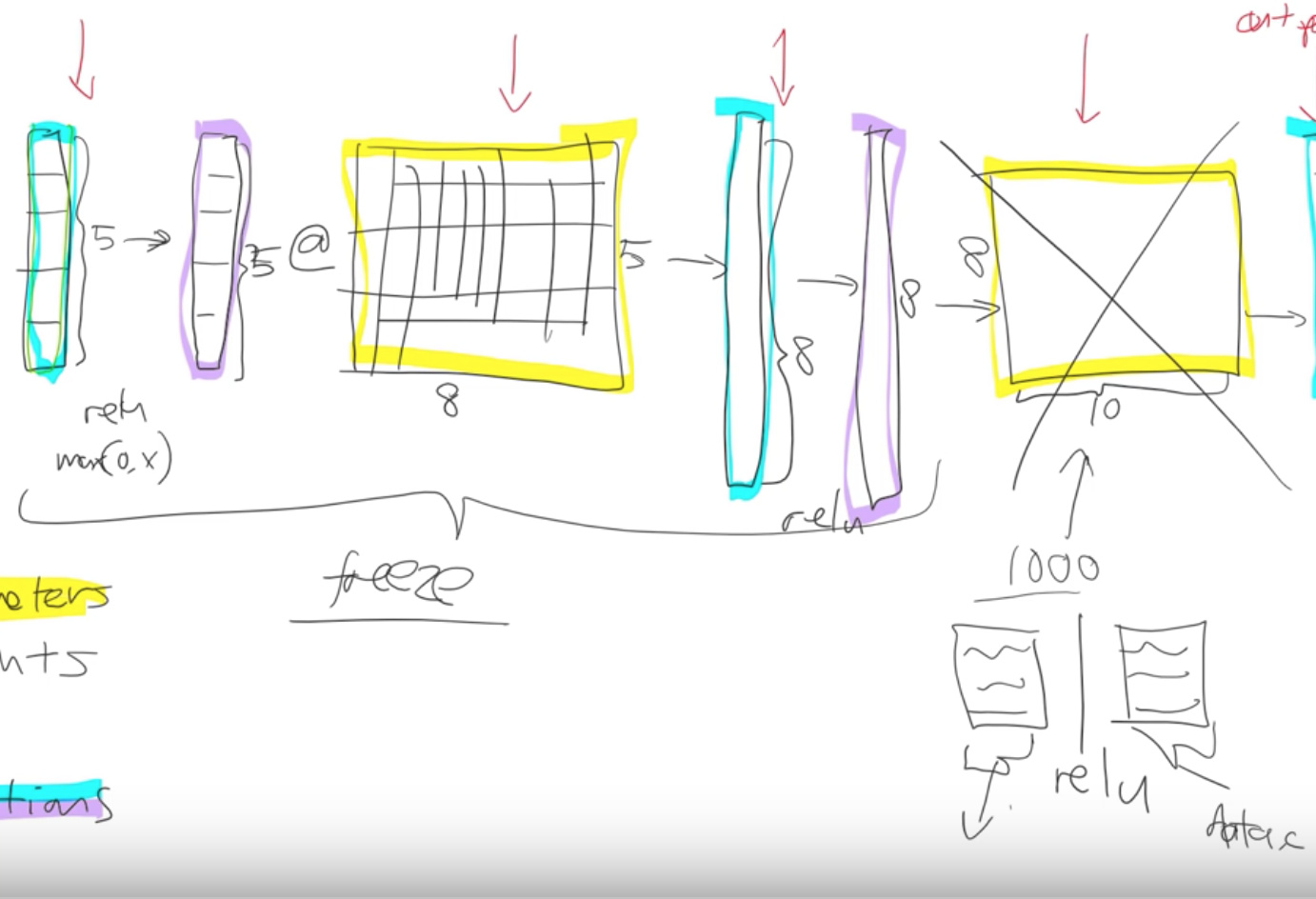
We definitely need to train these new weights because they’re random. Let’s not bother training any of the other weights at all. What we do when we freeze layers we are actually asking fastai and PyTorch that when we train however many epochs and when we call fit don’t backpropagate the gradients back into those layers.

In other words when you say

weights = weights  -  weights.grad * learning rate

Only do it for the new layers don’t bother doing it for the other layers. That is what freezing means.
Just don’t update those parameters. It’ll be a little bit faster because there are fewer calculations to do. It’ll take up a little bit less memory because there are fewer gradients that we have to store. But most importantly it’s not going to change weights that are already better than nothing. They’re better than random at the very least. that’s what happens when you call freeze. It doesn’t freeze the whole thing. It freezes everything except the randomly generated added layers that fastai puts on for us.

What happens next? After a while we say, this model is looking pretty good we probably should train the rest of the network now. So we unfreeze. Now we’re gonna train the whole thing but we still have a pretty good sense that these new layers we added to the end probably need more training and these ones right at the start that might just be like diagonal edges probably don’t need much training at all.

Discriminative Learning rates - forum question

[15:00]

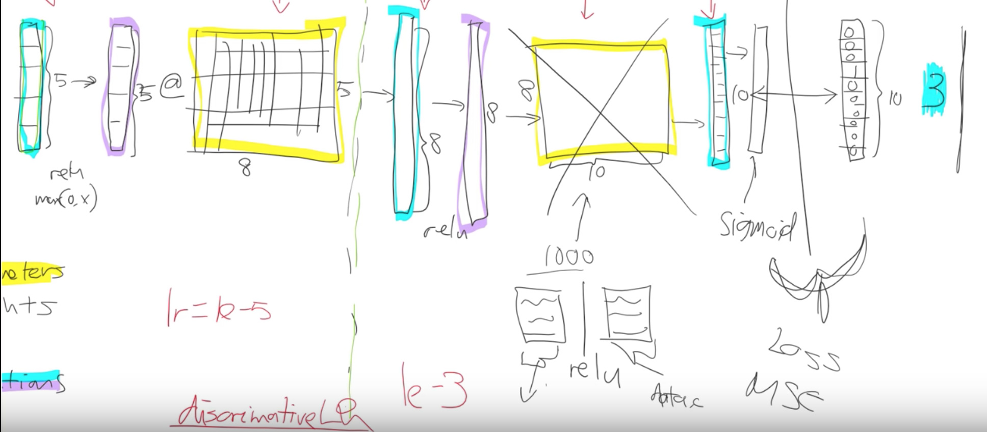
We split our model into a few sections. We say let’s give different parts of the model different learning rates.
Earlier layers of the model we might give a learning rate of 1e - 5 and newly added layers of the model we might give a learning rate of 1e - 3. What’s gonna happen now is that we can keep training the entire network. But because the learning rate for the early layers is smaller it’s going to move them around less because we think they’re already pretty good. If it’s already pretty good to the optimal value if you used a higher learning rate it could kick it out. It could actually make it worse which we really don’t want to happen.

This process is called using discriminative learning rates.

Fastai was the first one to use this technique. It’s starting to get more well-known slowly now. It’s a really important concept for transfer learning, without using this you just can’t get nearly as good results.

How do we do discriminative learning rates in fast AI?

[16:25]

Anywhere you can put a learning rate in fastai such as with the fit function.

You put in is the number of epochs
You put in is the learning rate.

Saying if you use fit one cycle the learning rate you can put a number of things that you can put.

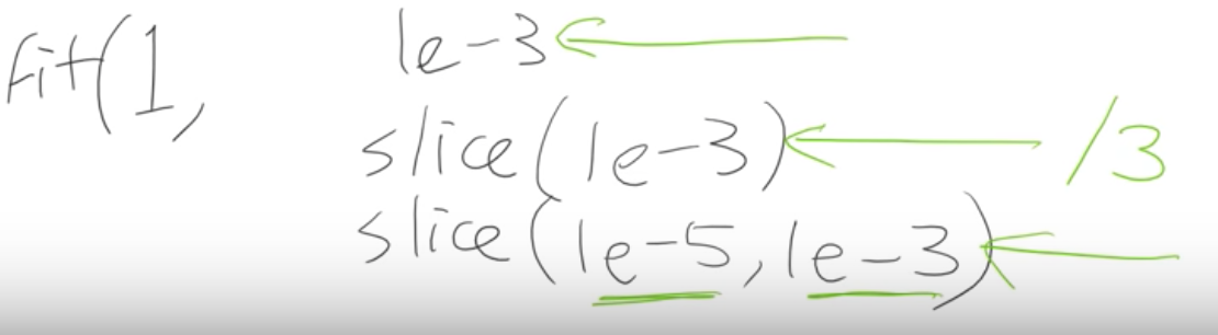
a single number like (1e - 3)
Just using a single number means every layer gets the same learning rate so you’re not using discriminative learning rates.
you can write a slice, for example, 1e -3 with a single number (1e-3)
If you pass a single number to slice it means the final layers get a learning rate of (1e - 3) and then all the other layers get the same learning rate which is that divided by 3. All of the other layers will be (1e - 3) / 3 and
the last layers will be 1e - 3.
You can write slice with two numbers, (1e-3, 1e -5)
In the last case, the final layers the these randomly hidden added layers will still be again 1e - 3.
The first layers will get 1e - 5. The other layers will get learning rates that are equally spread between those two. Multiplicatively equal. If there were three layers there would be (1e - 5), (1e - 4) and (1e-3). Equal multiples each time.

One slight tweak to make things a little bit simpler to manage we don’t actually give a different learning rate to every layer. We give a different learning rate to every layer group which is just we decided to put the groups together for you. So specifically what we do is the randomly added extra layers we call those one layer group. This is by default you can modify it and then all the rest. We split in half into two layer groups. So by default at least with a CNN, you’ll get three layer groups. If you say slice (1e-5, 1e - 3), you will get (1e - 5) learning rate for the first layer group. 1e- 4 for the second one and 1e - 3 for the third. So now if you go back and look at the way that we’re training hopefully you’ll see that this makes a lot of sense. This divided by 3 thing that is a little weird and we won’t talk about why that is until part two of the course. it is specific quirk around batch normalization. We can discuss that in the advanced topic.
This is fine-tuning.

Collaborative Filtering

[19:50]

lesson 4 collaborative filtering notebook

We were looking at collaborative filtering last week and in the collaborative filtering example we called fit_one_cycle(). We passed in just a single number.

learn.fit_one_cycle(3, 5e-3)

Total time: 00:04
epoch  train_loss  valid_loss
1      1.600185    0.962681    (00:01)
2      0.851333    0.678732    (00:01)
3      0.660136    0.666290    (00:01)

And that makes sense because in collaborative filtering we only have one layer there are a few different pieces in it. But there isn’t a matrix multiply followed by an activation function followed by another matrix multiply. Jeremy introduces another piece of jargon here. They’re not always exactly matrix multiplications. There’s something very similar to that. They’re linear functions that we add together. But the more general term for these things and that is written more general than matrix multiplications is affine functions.

If you hear Jeremy say the word affine function you can replace it in your head with matrix multiplication. But as we’ll see when we do convolutions. Convolutions are matrix multiplications where some of the weights are tied and so it would be slightly more accurate to call them affine functions.

Jeremy introduces a little bit more jargon each lesson so that when we read books or papers or watch other courses or read the documentation there will be more of the words we can recognize.

So when you see affine function it just means a linear function. It means something very close to matrix multiplication. Matrix multiplication is the most common kind affine function at least in deep learning.

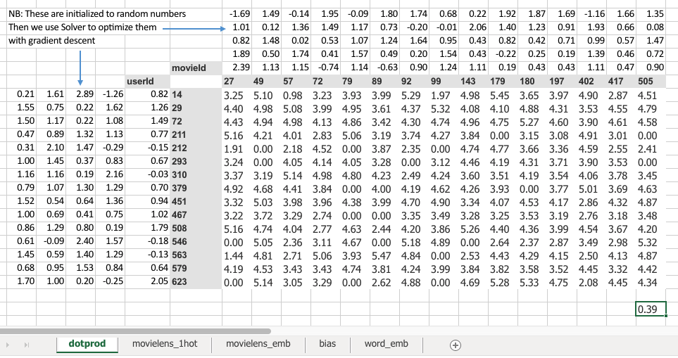
Collaborative Filtering in excel

collab_filter.xlsx

Primer

Specifically for collaborative filtering, the model we were using was movie ids and user ids from movie lens data.
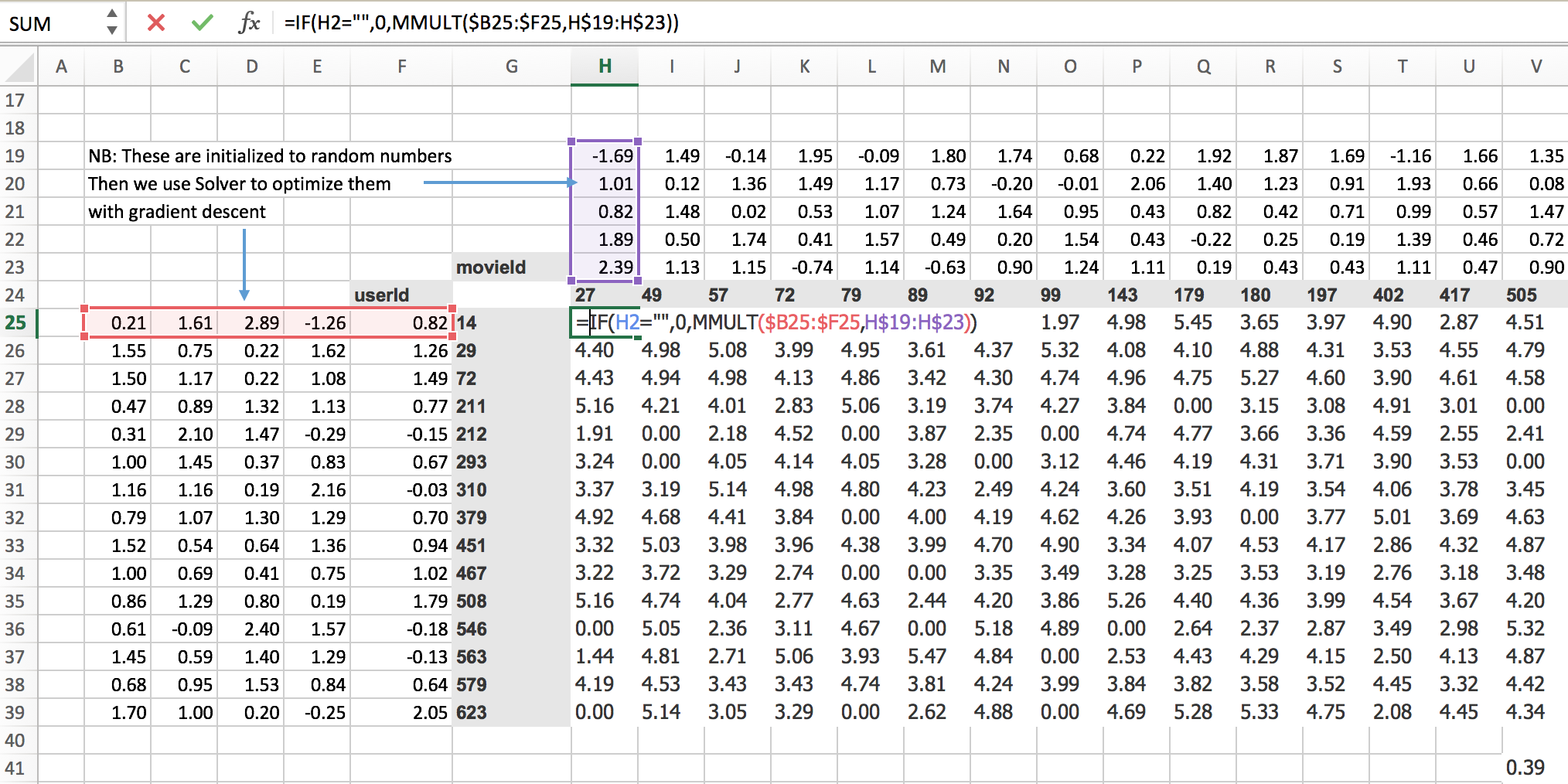
We predict for particular user say userId 14 will he like movie movieId 27? For this, we have to do some matrix multiplications. So Jeremy created some random metrics(5 random numbers) for each of moiveId and userId.

MovieIDs and their random matrices

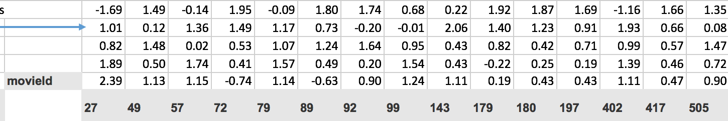
UserIDs and their random matrices

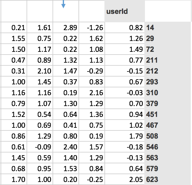
To know whether user 14 liked movie 27 we have to do the dot product of those random numbers associated with that particular userId and movieId.

Given that for userId, a random matrix is a row and that of movieId is the column. That’s the same as a matrix product so MMULT in Excel multiplies matrices.

=IF(H2="",0,MMULT($B25:$F25,H$19:H$23))
= 3.25

So 3.25 is the matrix product of those two.

Jeremy started this training last week by using solver in Excel. The average sum of squared .error got down to 0.39(Bottom right corner value).

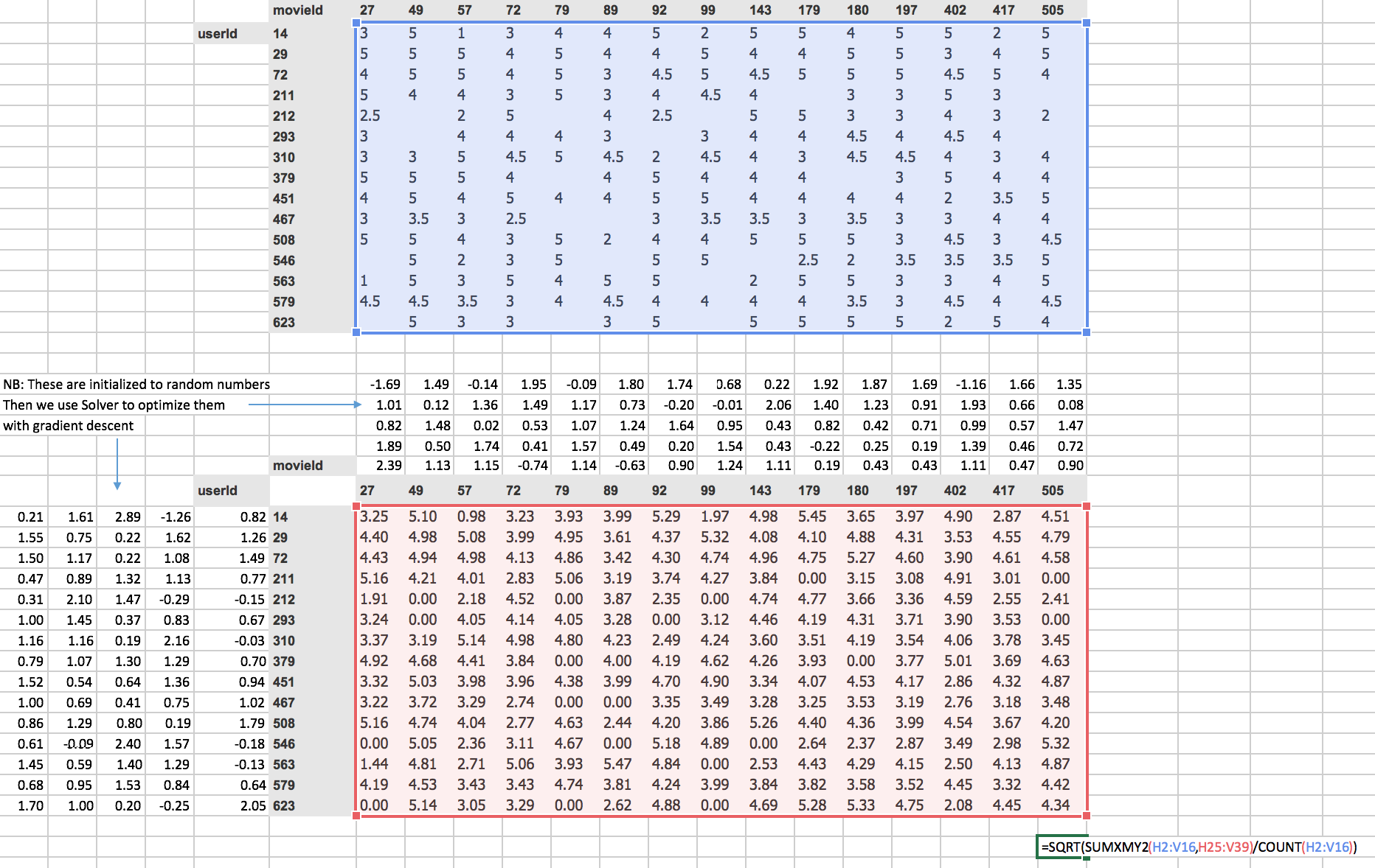
=SQRT(SUMXMY2(H2:V16,H25:V39)/COUNT(H2:V16))  
= 0.39

If we’re trying to predict something on a scale of 0.5 to 5 so on average we’re being wrong by about 0.4. That’s pretty good. You can see it’s pretty good if you look at ground truth values.

Ground truth
00%20PM

Predictions

55%20PM

like 3 ~= 3.25,
5 ~= 5.10 and
1~= 0.98
That’s pretty close. You got a general idea.

Embeddings

Then I started to talk about this idea of embedding matrices. In order to understand that, let’s put this worksheet aside and look at another worksheet named movielens_1hot tab.

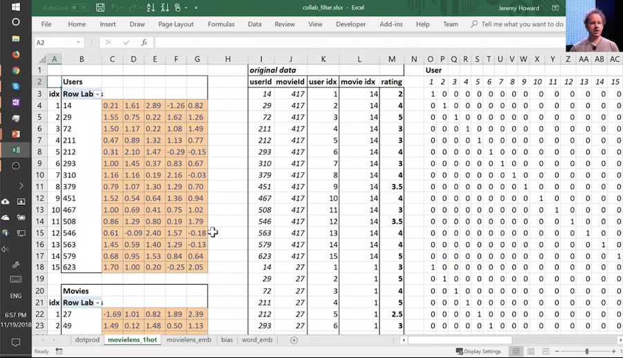
Here’s another worksheet. What I’ve done here is I have copied over those two weight matrices from the previous worksheet. Here’s the one for users, and here’s the one for movies. And the movies one I’ve transposed it, so it’s now got exactly the same dimensions as the users one.

So here are two weight matrices (in orange). Initially, they were random. We can train them with gradient descent. In the original data, the user IDs and movie IDs were numbers like these. To make life more convenient, I’ve converted them to numbers from 1 to 15 ( user_idx and movie_idx ). So in these columns, for every rating, I’ve got user ID movie ID rating using these mapped numbers so that they’re contiguous starting at one.

Now I’m going to replace user ID number 1 with this vector - the vector contains a 1 followed by 14 zeros. Then user number 2, I’m going to replace with a vector of 0 and then 1 and then 13 zeros. So movie ID 14, I’ve also replaced with another vector which is 13 zeros and then a 1 and then a 0. These are called one-hot encodings, by the way. This is not part of a neural net. This is just like some input pre-processing where I’m literally making this my new input

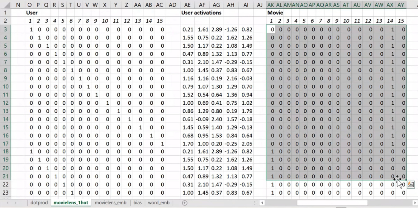
So this is my new inputs for my movies, this is my new inputs for my users. These are the inputs to a neural net.

What I’m going to do now is I’m going to take this input matrix and I’m going to do a matrix multiplied by the weight matrix. That’ll work because the weight matrix has 15 rows, and this (one-hot encoding) has 15 columns. I can multiply those two matrices together because they match. You can do matrix multiplication in Excel using the MMULT function. Just be careful if you’re using Excel. Because this is a function that returns multiple numbers, you can’t just hit enter when you finish with it; you have to hit ctrl+shift+enter. ctrl+shift+enter means this is an array function - something that returns multiple values.

Here (User activations) is the matrix product of this input matrix of inputs, and this parameter matrix or weight matrix. So that’s just a normal neural network layer. It’s just a regular matrix multiply. So we can do the same thing for movies, and so here’s the matrix multiply for movies.

Well, here’s the thing. This input, we claim, is this one hot encoded version of user ID number 1, and these activations are the activations for user ID number one. Why is that? Because if you think about it, the matrix multiplication between one hot encoded vector and some matrix is actually going to find the Nth row of that matrix when the one is in position N. So what we’ve done here is we’ve actually got a matrix multiply that is creating these output activations. But it’s doing it in a very interesting way - it’s effectively finding a particular row in the input matrix.

Having done that, we can then multiply those two sets together (just a dot product), and we can then find the loss squared, and then we can find the average loss.

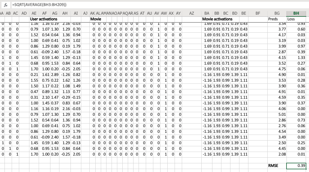
And lo and behold, that number 0.39 is the same as this number (from the solver) because they’re doing the same thing.

This one (“dotprod” version) was finding this particular users embedding vector, this one (“movielens_1hot” version) is just doing a matrix multiply, and therefore we know they are mathematically identical .

Embedding once again [27:56]

So let’s lay that out again. Here’s our final version

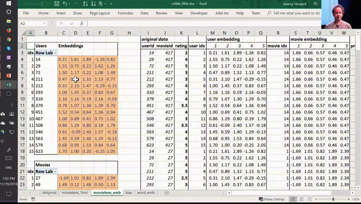
This is the same weight matrices again - exactly the same I’ve copied them over. And here’s those user IDs and movie IDs again. But this time, I’ve laid them out just in a normal tabular form just like you would expect to seein the input to your model. And this time, I have got exactly the same set of activations here (user embedding) that I had in movielens_1hot. But in this case I’ve calculated these activations using Excels OFFSET function which is an array look up. This version ( movielens_emb ) is identical to movielens_1hot version, but obviously it’s much less memory intensive and much faster because I don’t actually create the one hot encoded matrix and I don’t actually do a matrix multiply. That matrix multiply is nearly all multiplying by zero which is a total waste of time.

So in other words, multiplying by a one hot encoded matrix is identical to doing an array lookup. Therefore we should always do the array lookup version , and therefore we have a specific way of saying I want to do a matrix multiplication by a one hot encoded matrix without ever actually creating it. I’m just instead going to pass in a bunch of integers and pretend they’re one not encoded. And that is called an embedding .

You might have heard this word “embedding” all over the places as if it’s some magic advanced mathy thing, but embedding means look something up in an array. But it’s interesting to know that looking something up in an array is mathematically identical to doing a matrix product by a one hot encoded matrix. And therefore, an embedding fits very nicely in our standard model of our neural networks work.

Now suddenly it’s as if we have another whole kind of layer. It’s a kind of layer where we get to look things up in an array. But we actually didn’t do anything special. We just added this computational shortcut - this thing called an embedding which is simply a fast memory efficient way of multiplying by hot encoded matrix.

So this is really important. Because when you hear people say embedding, you need to replace it in your head with “an array lookup” which we know is mathematically identical to matrix multiply by a one hot encoded matrix.

Here’s the thing though, it has kind of interesting semantics. Because when you do multiply something by a one hot encoded matrix, you get this nice feature where the rows of your weight matrix, the values only appear (for row number one, for example) where you get user ID number one in your inputs. So in other words you kind of end up with this weight matrix where certain rows of weights correspond to certain values of your input. And that’s pretty interesting. It’s particularly interesting here because (going back to a kind of most convenient way to look at this) because the only way that we can calculate an output activation is by doing a dot product of these two input vectors. That means that they kind of have to correspond with each other. There has to be some way of saying if this number for a user is high and this number for a movie is high, then the user will like the movie. So the only way that can possibly make sense is if these numbers represent features of personal taste and corresponding features of movies . For example, the movie has John Travolta in it and user ID likes John Travolta, then you’ll like this movie.

We’re not actually deciding the rows mean anything. We’re not doing anything to make the rows mean anything. But the only way that this gradient descent could possibly come up with a good answer is if it figures out what the aspects of movie taste are and the corresponding features of movies are. So those underlying kind of features that appear that are called latent factors or latent features . They’re these hidden things that were there all along, and once we train this neural net, they suddenly appear.

Bias [33:08]

Now here’s the problem. No one’s going to like Battlefield Earth. It’s not a good movie even though it has John Travolta in it. So how are we going to deal with that? Because there’s this feature called I like John Travolta movies, and this feature called this movie has John Travolta, and so this is now like you’re gonna like the movie. But we need to save some way to say “unless it’s Battlefield Earth” or “you’re a Scientologist” - either one. So how do we do that? We need to add in bias .

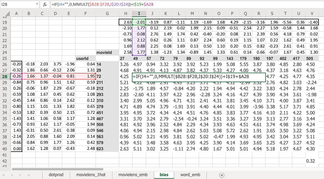
Here is the same thing again, the same construct, same shape of everything. But this time you’ve got an extra row. So now this is not just the matrix product of that and that, but I’m also adding on this number and this number. Which means, now each movie can have an overall “this is a great movie” versus “this isn’t a great movie” and every user can have an overall “this user rates movies highly” or “this user doesn’t rate movies highly” - that’s called the bias. So this is hopefully going to look very familiar. This is the same usual linear model concept or linear layer concept from a neural net that you have a matrix product and a bias.

And remember from lesson 2 SGD notebook, you never actually need a bias. You could always just add a column of ones to your input data and then that gives you bias for free, but that’s pretty inefficient. So in practice, all neural networks library explicitly have a concept of bias. We don’t actually add the column of ones.

So what does that do? Well just before I came in today, I ran data solver on this as well, and we can check the RMSE. So the root mean squared here is 0.32 versus the version without bias was 0.39. So you can see that this slightly better model gives us a better result. And it’s better because it’s giving both more flexibility and it also just makes sense semantically that you need to be able to say whether I’d like the movie is not just about the combination of what actors it has, whether it’s dialogue-driven, and how much action is in it but just is it a good movie or am i somebody who rates movies highly.

So there’s all the pieces of this collaborative filtering model.

Question : When we load a pre-trained model, can we explore the activation grids to see what they might be good at recognizing? [36:11]

Yes, you can. And we will learn how to (should be) in the next lesson.

Question : Can we have an explanation of what the first argument in fit_one_cycle actually represents? Is it equivalent to an epoch?

Yes, the first argument to fit_one_cycle or fit is number of epochs. In other words, an epoch is looking at every input once. If you do 10 epochs, you’re looking at every input ten times. So there’s a chance you might start overfitting if you’ve got lots of lots of parameters and a high learning rate. If you only do one epoch, it’s impossible to overfit, and so that’s why it’s kind of useful to remember how many epochs you’re doing.

Question : What is an affine function?

An affine function is a linear function. I don’t know if we need much more detail than that. If you’re multiplying things together and adding them up, it’s an affine function. I’m not going to bother with the exact mathematical definition, partly because I’m a terrible mathematician and partly because it doesn’t matter. But if you just remember that you’re multiplying things together and then adding them up, that’s the most important thing. It’s linear. And therefore if you put an affine function on top of an affine function, that’s just another affine function. You haven’t won anything at all. That’s a total waste of time. So you need to sandwich it with any kind of non-linearity pretty much works - including replacing the negatives with zeros which we call ReLU. So if you do affine, ReLU, affine, ReLU, affine, ReLU, you have a deep neural network.

[38:25]

Let’s go back to the collaborative filtering notebook. And this time we’re going to grab the whole Movielens 100k dataset. There’s also a 20 million dataset, by the way, so really a great project available made by this group called GroupLens. They actually update the Movielens datasets on a regular basis, but they helpfully provide the original one. We’re going to use the original one because that means that we can compare to baselines. Because everybody basically they say, hey if you’re going to compare the baselines make sure you all use the same dataset, here’s the one you should use. Unfortunately, it means that we’re going to be restricted to movies that are before 1998. So maybe you won’t have seen them all. but that’s the price we pay. You can replace this with ml-latest when you download it and use it if you want to play around with movies that are up to date.

path=Path('data/ml-100k/')

The original Movielens dataset, the more recent ones are in a CSV file it’s super convenient to use. The original one is slightly messy. First of all, they don’t use commas for delimiters, they use tabs. So in Pandas, you can just say what’s the delimiter and you loaded in. The second is they don’t add a header row so that you know what column is what, so you have to tell Pandas there’s no header row. Then since there’s no header row, you have to tell Pandas what are the names of four columns. Rather than that, that’s all we need.

ratings = pd.read_csv(path/'u.data', delimiter='\t', header=None, names=[user,item,'rating','timestamp']) ratings.head()

	userId	movieId	rating	timestamp
0	196	242	3	881250949
1	186	302	3	891717742
2	22	377	1	878887116
3	244	51	2	880606923
4	166	346	1	886397596

So we can then have a look at head which remember is the first few rows and there is our ratings; user, movie, rating.

Let’s make it more fun. Let’s see what the movies actually are.

movies = pd.read_csv(path/'u.item',  delimiter='|', encoding='latin-1', header=None,
                 names=[item, 'title', 'date', 'N', 'url', *[f'g{i}' for i in range(19)]])
movies.head()

	movieId	title	date	N	url	g1	g2	g3	g4	…	g16
0	1	Toy Story (1995)	01-Jan-1995	NaN	http://us.imdb.com/M/title-exact?Toy%20Story%2…	0	0	1	1	…	0
1	2	GoldenEye (1995)	01-Jan-1995	NaN	http://us.imdb.com/M/title-exact?GoldenEye%20(…	1	1	0	0	…	1
2	3	Four Rooms (1995)	01-Jan-1995	NaN	http://us.imdb.com/M/title-exact?Four%20Rooms%…	0	0	0	0	…	1
3	4	Get Shorty (1995)	01-Jan-1995	NaN	http://us.imdb.com/M/title-exact?Get%20Shorty%…	1	0	0	0	…	0
4	5	Copycat (1995)	01-Jan-1995	NaN	http://us.imdb.com/M/title-exact?Copycat%20(1995)	0	0	0	0	…	1

I’ll just point something out here, which is there’s this thing called encoding= . I’m going to get rid of it and I get this error:

---------------------------------------------------------------------------
UnicodeDecodeError                        Traceback (most recent call last)
pandas/_libs/parsers.pyx in pandas._libs.parsers.TextReader._convert_tokens()
pandas/_libs/parsers.pyx in pandas._libs.parsers.TextReader._convert_with_dtype()
pandas/_libs/parsers.pyx in pandas._libs.parsers.TextReader._string_convert()
pandas/_libs/parsers.pyx in pandas._libs.parsers._string_box_utf8()

UnicodeDecodeError: 'utf-8' codec can't decode byte 0xe9 in position 3: invalid continuation byte

During handling of the above exception, another exception occurred:
UnicodeDecodeError                        Traceback (most recent call last)
<ipython-input-15-d6ba3ac593ed> in <module>
      1 movies = pd.read_csv(path/'u.item',  delimiter='|', header=None,
----> 2                     names=[item, 'title', 'date', 'N', 'url', *[f'g{i}' for i in range(19)]])
      3 movies.head()

~/src/miniconda3/envs/fastai/lib/python3.6/site-packages/pandas/io/parsers.py in parser_f(filepath_or_buffer, sep, delimiter, header, names, index_col, usecols, squeeze, prefix, mangle_dupe_cols, dtype, engine, converters, true_values, false_values, skipinitialspace, skiprows, nrows, na_values, keep_default_na, na_filter, verbose, skip_blank_lines, parse_dates, infer_datetime_format, keep_date_col, date_parser, dayfirst, iterator, chunksize, compression, thousands, decimal, lineterminator, quotechar, quoting, escapechar, comment, encoding, dialect, tupleize_cols, error_bad_lines, warn_bad_lines, skipfooter, doublequote, delim_whitespace, low_memory, memory_map, float_precision)
    676                     skip_blank_lines=skip_blank_lines)
    677 
--> 678         return _read(filepath_or_buffer, kwds)
    679 
    680     parser_f.__name__ = name

~/src/miniconda3/envs/fastai/lib/python3.6/site-packages/pandas/io/parsers.py in _read(filepath_or_buffer, kwds)
    444 
    445     try:
--> 446         data = parser.read(nrows)
    447     finally:
    448         parser.close()

~/src/miniconda3/envs/fastai/lib/python3.6/site-packages/pandas/io/parsers.py in read(self, nrows)
   1034                 raise ValueError('skipfooter not supported for iteration')
   1035 
-> 1036         ret = self._engine.read(nrows)
   1037 
   1038         # May alter columns / col_dict

~/src/miniconda3/envs/fastai/lib/python3.6/site-packages/pandas/io/parsers.py in read(self, nrows)
   1846     def read(self, nrows=None):
   1847         try:
-> 1848             data = self._reader.read(nrows)
   1849         except StopIteration:
   1850             if self._first_chunk:

pandas/_libs/parsers.pyx in pandas._libs.parsers.TextReader.read()
pandas/_libs/parsers.pyx in pandas._libs.parsers.TextReader._read_low_memory()
pandas/_libs/parsers.pyx in pandas._libs.parsers.TextReader._read_rows()
pandas/_libs/parsers.pyx in pandas._libs.parsers.TextReader._convert_column_data()
pandas/_libs/parsers.pyx in pandas._libs.parsers.TextReader._convert_tokens()
pandas/_libs/parsers.pyx in pandas._libs.parsers.TextReader._convert_with_dtype()
pandas/_libs/parsers.pyx in pandas._libs.parsers.TextReader._string_convert()
pandas/_libs/parsers.pyx in pandas._libs.parsers._string_box_utf8()

UnicodeDecodeError: 'utf-8' codec can't decode byte 0xe9 in position 3: invalid continuation byte

Lankinen · December 20, 2018, 1:22pm

Thank you for creating again these create notes. Here is mine a little bit late.

dinesh.chauhan · March 7, 2019, 6:07pm

Is there any extension for these notes ? Where do I see Embeddings part discussed ?

PoonamV · March 8, 2019, 6:17am

@sgugger Can you please turn this post into a wiki. I can’t edit it anymore. Thanks.

sgugger · March 8, 2019, 2:54pm

Just did.

johnri99 · August 12, 2019, 1:51pm

Thanks, very useful notes. About the only place I could find an explantation as to what slice did when you only provided one value