<<< Notes: Lesson 3 | Notes: Lesson 5 >>>
Hi everybody, welcome to lesson 4.

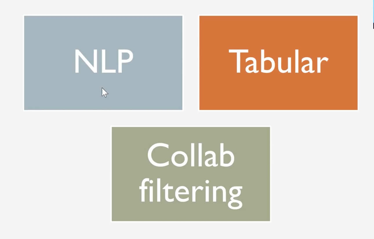
We are going to finish our journey through these key applications. We already looked at a range of computer vision applications like image classification, localization, regression etc. We slightly touched NLP. we are gonna take a deeper dive into NLP and transfer Learning today. We are going to then look at tabular data and collaborative filtering, which are both super useful applications.
Then we are going to dig deeper into collaborative filtering to see exactly what’s happening mathematically. What’s happening on the computer.
And we are going to use that to go back gradually in reverse order through the applications again to understand exactly what’s going on behind the scenes in all of those applications.
Important posts to watch:
Software Update
![]() Always remember to do an update on fast.ai library and course repo.
Always remember to do an update on fast.ai library and course repo.
conda install -c fastai fastai for the library update
git pull for the course repo update.
Lesson 4 Notebooks:
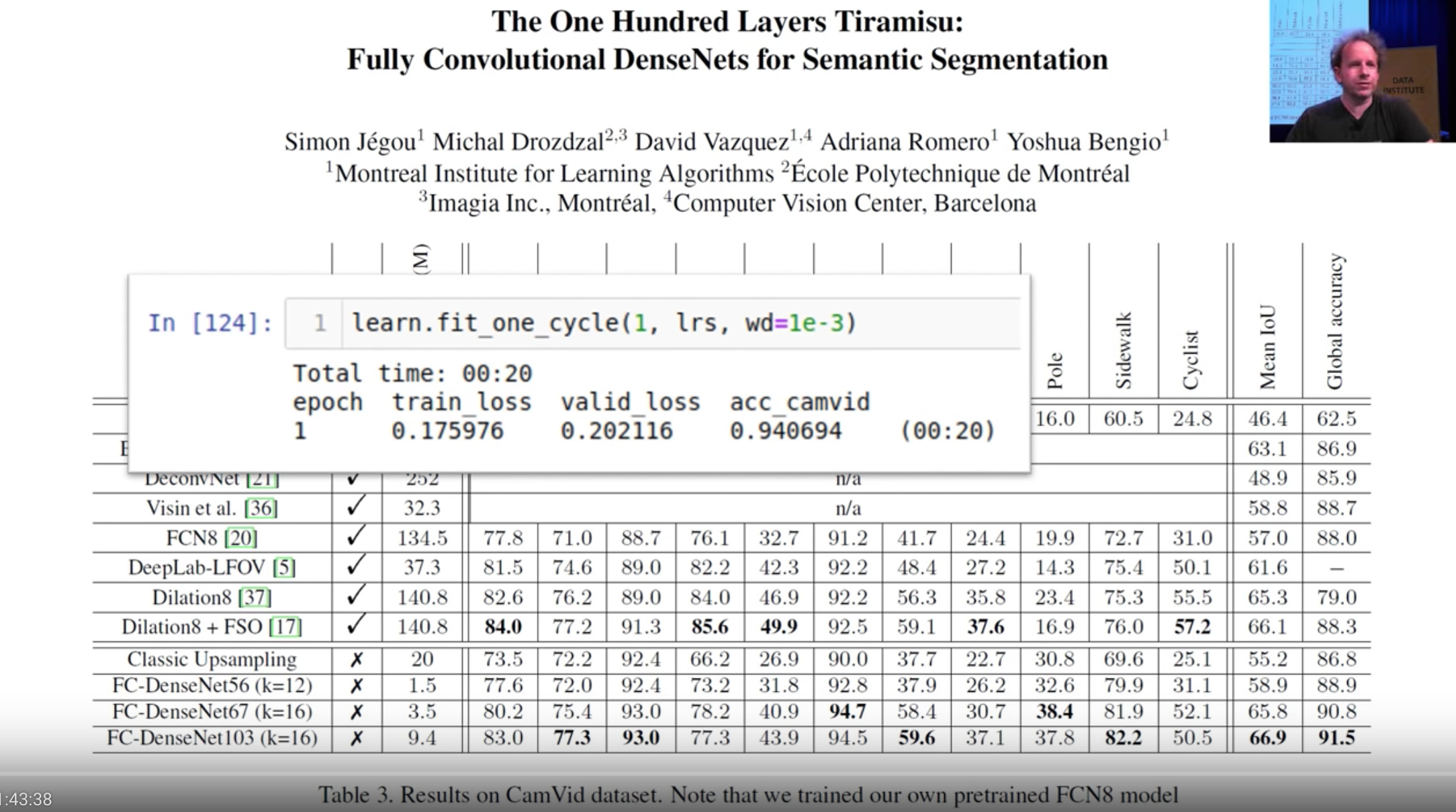
CamVid Benchmark Clarity
SOTA for CamVid we compared last week was not a fair comparison Because paper actually used a small subset of classes and we used all of the classes. So Jason in the study group was kind enough to re-run the experiment with the exact number of classes from the paper and our accuracy went up to 94% compared to 91.5%in the paper. This is a cool example of how by using pretty much default we can go beyond SOTA year or 2 ago.
NLP - a quick review
NLP is Natural Language Processing. It’s about taking text and doing something with it. And one of the applications of NLP test classification is a particularly useful, practically useful application that we gonna start focusing on. Classifying text or document can be used for anything from spam prevention to identifying fake news to finding a diagnosis to medical reports, finding mentions of your product on twitter etc.
It’s pretty much interesting.
Classifying legal text
Actually, there was a great example during the week from one of the fast.ai students who is a lawyer, who mentioned on the forums he got good results from classifying legal texts using this NLP approach.
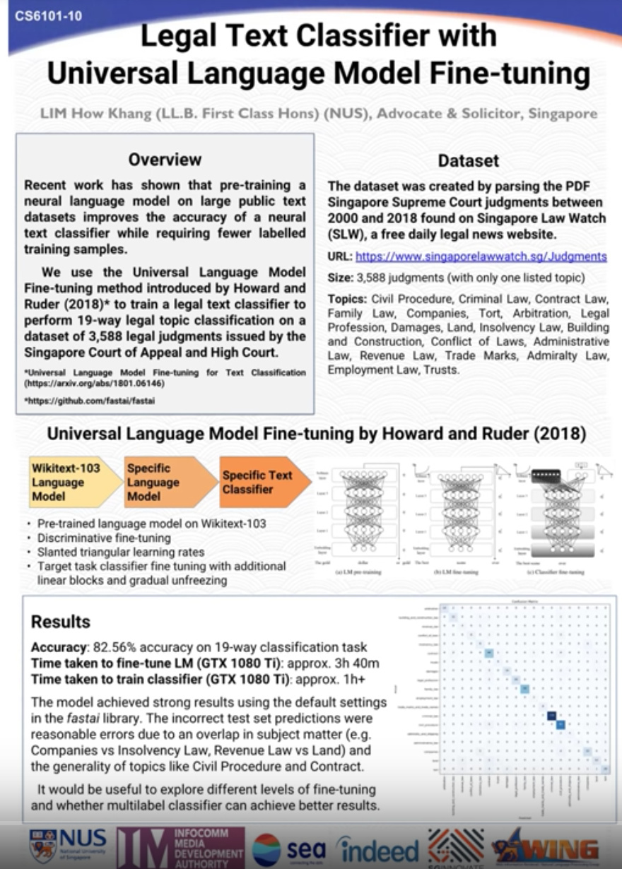
Above is technical post they presented in academic conference describing the approach.
And these series of three steps, and classification matrix you can recognize.
We are going to understand those three steps today.
IMDB movie reviews Sentiment Classification
We are going to start with this movie review. and decide whether it’s positive or negative.
Viewer’s sentiment about a movie.
But here is the problem, we have in the training set 25000 movie reviews. For each one, we have like 1 bit of information, they liked it or they didn’t like it. In today’s lesson, we will learn more about this.
What is a Neural Network:
Remember these are a bunch of matrix multiplications and simple nonlinearities particularly replacing negatives with zeros(relu function). Those weight matrices start out random. So if we start out with random parameters and train them to recognize positive versus negative movie reviews. You have 25000 reviews that mean 25000 1 and 0s to tell you ‘I like this one’ or ‘I don’t like that one’.
This is clearly not enough information to learn basically how to speak English. How to speak English well enough to recognize they liked it or didn’t. Sometimes there can be new words. In the case of online movie reviews like IMDB people can use sarcasm. It can be really quite tricky.
For a long time till recent times until this year, Neural nets dint do a good job at all at this kind of classification problem. And that was right there is not enough information available. So the trick hopefully you can all guess is to use Transfer Learning. It’s always the trick.
Last year in this course Jeremy tries something crazy. He tried transfer learning on NLP to demonstrate if that can work and it actually worked extraordinarily well. So here we are a year later.
And transfer learning in NLP is absolutely the hit thing now.
What happens in transfer learning?
The key thing is we gonna start with the same thing we used for computer vision a pre-trained model, that has been trained to do something different than what we are doing with it. So for Imagenet, that was originally built as a model to predict 1000 categories of each photo falls into and people then fine-tuned it to their own problems So we going to start with a pre-trained model that was going to do something else, not a movie review classification. This pre-trained model which is called a language model
what is the language model?
It has a very specific meaning. A language model is something which predicts next word in a sentence. To predict next word in a sentence you need to know quite a lot about the English language. Assuming you are doing it in English language and quite a lot world knowledge. By world knowledge Jeremy means
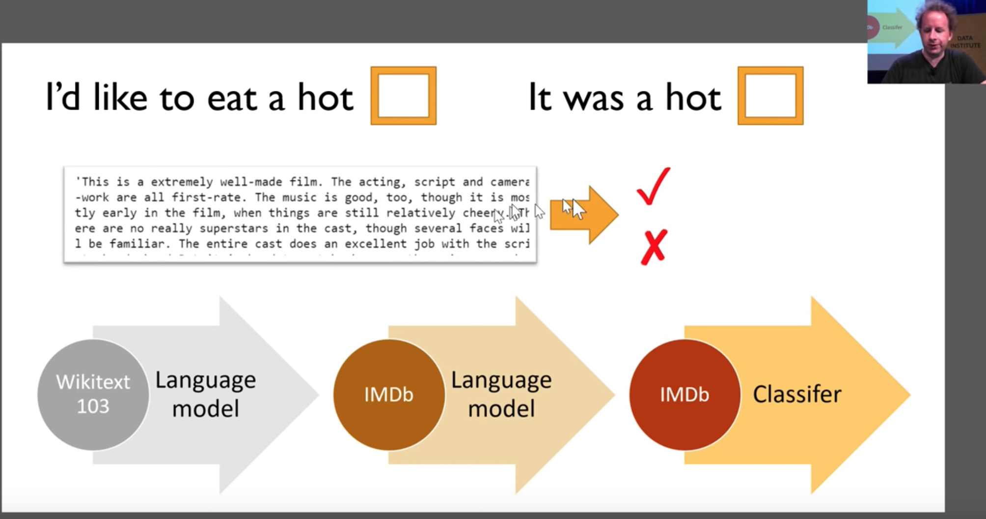
For example, complete the below sentences using your language model.
- I’d like to eat a hot _______?(dog)
- It was a hot _____? (day.)
Previous approaches to NLP used Ngrams largely. Ngrams means how often these pairs or triplets of word occur next to each other. Ngrams are terrible here because there is not enough information here to decide what the next word probably is. But with the neural net, you absolutely can.
If you train a neural net to predict next word in a sentence, then you actually have a lot of information, Rather than having a single bit for every 2000 movie reviews, liked it or didn’t like it. Every single word you can try and predict the next word. So in a 2000 words movie review, there are 1999 opportunities to predict the next word. Better still you don’t just need to look at movie reviews. The hard thing isn’t so much about does this person liked the movie or not but how do you speak English, So you can learn how you speak English roughly by some much bigger set of documents. So what Jeremy did, he started with Wikipedia. Stephen Merity and some other colleagues built the Wikitext-103 dataset, which is a subset of most of largest articles from Wikipedia with a little bit of processing, that’s available for download. So basically grabbing Wikipedia. Jeremy built a language model on whole of Wikipedia. So Jeremy built a neural net, which will predict next word in every significantly sized Wikipedia article. And that’s a lot of information. Something like billions of tokens. So we got billions of words to predict, we make mistakes in those predictions, we get gradients from that, we can update our weights and we can try to get better and better until we get pretty good at predicting next words in Wikipedia.
Why is that useful? Because at that point we have got a model that knows how to complete sentences like this. So it knows quite a lot about English and a lot about how the world works. What kinds of things tend to be hot in different situations, for instance.
Ideally, it would learn things like in 1996 in a speech to the United Nations, United States President ______ said…
That will be a really good language model because it needs to know who was the president in that year.
Getting really good at training language model is a great way to learn or teach a neural net a lot about what is our world, what’s in our world or how do things work in our world. It’s really a fascinating topic.
3 step process described
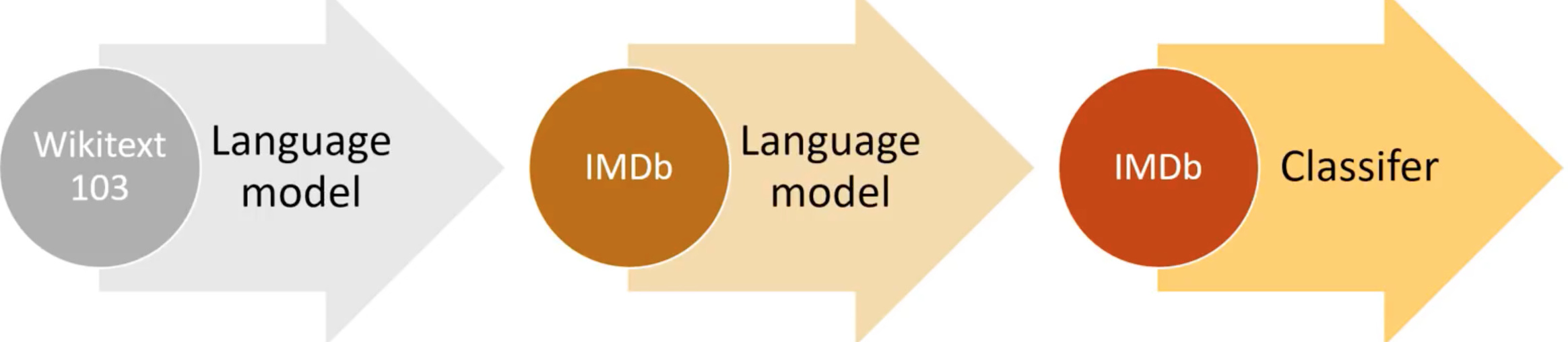
1. Wikitext-103 - A language model
You can start by training a language model on all of the Wikipedia and then we can make that available to all of you just like a pre-trained Imagenet model for the vision we have now pre-trained wikitext model for NLP.
Not because it’s particularly useful of itself, predicting next word of a sentence is somewhat useful but not normally what we want to do But it tells us its a model that understands a lot about English language and a lot about what language describes.
2. IMDB - Transfer Learning.
We can take the language model trained on wikitext-103 and use that as a transfer learning to create a new language model that’s specifically good at predicting the next word in movie reviews. If we can build such a model, pre-trained with wikitext then that’s gonna understand a lot about “my favorite actor is Tom _____(who)?” or “I thought photography was fantastic but I didn’t like the _____(director)”.
Its gonna learn more about specifically how movie reviews are written. It will even learn what are the names of popular movies. So that means we can use a huge corpus of movie reviews even if we don’t know if they are positive or negative. It will learn how movie reviews are written. So all of this pre-training, and all of this language model fine-tuning we don’t need any labels at all. It’s what the researcher Yann Lekun calls self-supervised learning.
In other words, it’s a classic supervised model, we have labels, but the labels are not somebody else has created, they are in kind of built into the dataset itself. So this is really neat.
So now we have got something that is good at understanding movie reviews.
3. IMDB -The classifier
Now we can use this language model to fine-tune the thing we want to do. In this case to classify a movie review to be positive or negative. So last year Jeremy thought, 25000 1s and 0s would be enough feedback to fine-tune that model. And it turned out, it absolutely was.
Question:
[12:48]
Does the language model approach works for texts in forums which have informal English like misspelled words, slang or short forms like S6 instead of Samsung S6?
Yes, It does. Particularly, If you start with your wikitext model and fine tune it with your data we call it a target corpus. Corpus is a bunch of documents like emails. tweets or medical reports etc. So you could fine-tune it. So it can learn specifics about slang, that didn’t appear in the full corpus. And this is what people were most surprised about when Jeremy did research last year. They thought learning from Wikipedia wouldn’t be that helpful because that’s is not how people tend to write.
But it turned out pretty much helpful because there is much difference between Wikipedia and random words than there is between Wikipedia and Reddit. So it kind of gets you 99% of the way there.
Swiftkey
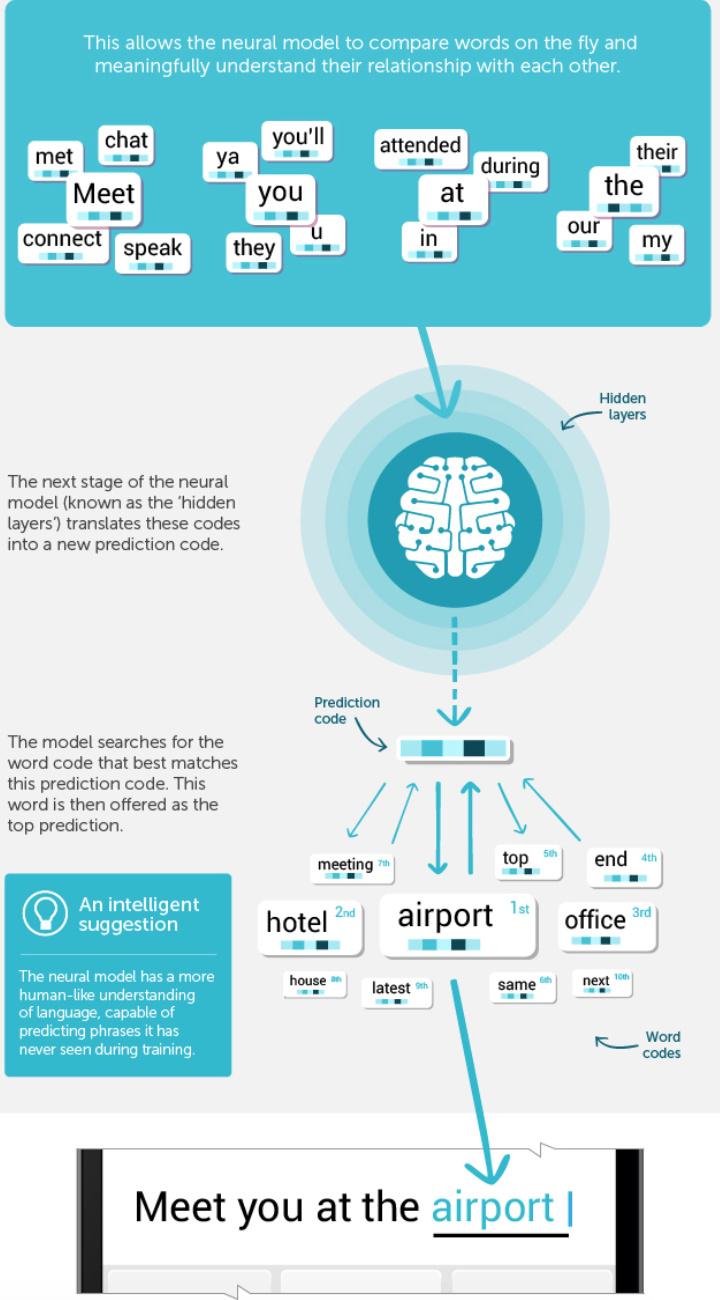
So these language models are kind of powerful. For example, there was a blog post from a Swiftkey, which does mobile phone predictive text modeling. They describe how they rewrote their underlying model to use the neural network. This was a year or two ago. Now, most of the phone keyboards do this. You will be typing on your mobile and in suggested prediction, there is something that says what word you wanna write next.
So, that’s a language model in your phone.
LaTex Generator
Another example was the researcher Andrej Karpathy who now runs all this stuff at Tesla, back when he was a Ph.D. student, he created a language model of text in LaTeX documents and created this automatic generation of LaTeX documents that then became these automatically generated papers. That’s pretty cute.
We’re not really that interested in the output of the language model ourselves. We’re just interested in it because it’s helpful with this process.
Basic process of Text Classification [15:13]
We briefly looked at the process last week. The basic process is, we’re going to start with the data in some format. So for example, we’ve prepared a little IMDB sample that you can use which is in CSV file. You can read it in with Pandas and there’s negative or positive, the text of each movie review, and boolean of is it in the validation set or the training set.
path = untar_data(URLs.IMDB_SAMPLE)
path.ls()
Out[ ]:
[PosixPath('/home/jhoward/.fastai/data/imdb_sample/texts.csv'),
 PosixPath('/home/jhoward/.fastai/data/imdb_sample/models'),
 PosixPath('/home/jhoward/.fastai/data/imdb_sample/export.pkl')]

df = pd.read_csv(path/'texts.csv')
df.head()

label	text	is_valid
0	negative	Un-bleeping-believable! Meg Ryan doesn't even ...	False
1	positive	This is an extremely well-made film. The acting...	False
2	negative	Every once in a long while a movie will come a...	False
3	positive	Name just says it all. I watched this movie wi...	False
4	negative	This movie succeeds at being one of the most u...	False

df['text'][1]
Out[ ]:
'This is an extremely well-made film. The acting, script, and camera-work are all first-rate. The music is good, too, though it is mostly early in the film, when things are still relatively cheery...'
You can just go TextDataBunch.from_csv() to grab a language model specific data bunch.
data_lm = TextDataBunch.from_csv(path, 'texts.csv')
And then you can create a learner from that in the usual way and fit it.
data_lm.save()
You can save the data bunch which means that the pre-processing that is done, you don’t have to do it again. You can just lo
data = TextDataBunch.load(path)
What happens behind the scenes if we now load it as a classification data bunch (that’s going to allow us to see the labels as well)?
data = TextClasDataBunch.load(path)
data.show_batch()
| text | target |
|---|---|
| xxbos xxfld 1 xxmaj raising xxmaj victor xxmaj vargas : a xxmaj review \n\n xxmaj you know , xxmaj raising xxmaj victor xxmaj vargas is like sticking your hands into a big , xxunk bowl of xxunk . xxmaj it 's warm and gooey , but you 're not sure if it feels right . xxmaj try as i might , no matter how warm and gooey xxmaj raising xxmaj | negative |
As we described, it basically creates a separate unit (i.e. a “token”) for each separate part of a word. So most of them are just for words, but sometimes if it’s like an 's from it’s, it will get its own token. Every bit of punctuation tends to get its own token (a comma, a full stop, and so forth).
Then the next thing that we do is a numericalization which is where we find what are all of the unique tokens that appear here, and we create a big list of them. Here’s the first ten in order of frequency:
data.vocab.itos[:10]
['xxunk', 'xxpad', 'the', ',', '.', 'and', 'a', 'of', 'to', 'is']
And that big list of unique possible tokens is called the vocabulary which we just call it a “vocab”. So what we then do is we replace the tokens with the ID of where is that token in the vocab
data.train_ds[0][0]

Text xxbos xxfld 1 he now has a name , an identity , some memories and a a lost girlfriend . all he wanted was to disappear , but still , they xxunk him and destroyed the world he hardly built . now he wants some explanation , and to get ride of the people how made him what he is . yeah , jason bourne is back , and this time , he 's here with a vengeance .

data.train_ds[0][0].data[:10]
array([ 43,  44,  40,  34, 171,  62,   6, 352,   3,  47])
That’s numericalization. Here’s the thing though. As you’ll learn, every word in our vocab is going to require a separate row in a weight matrix in our neural net. So to avoid that weight matrix getting too huge, we restrict the vocab to no more than (by default) 60,000 words. And if a word doesn’t appear more than two times, we don’t put it in the vocab either. So we keep the vocab to a reasonable size in that way. When you see these xxunk, that’s an unknown token. It just means this was something that was not a common enough word to appear in our vocab.
We also have a couple of other special tokens like (see fastai.text.transform.py for up-to-date info):
xxfld: This is a special thing where if you’ve got like title, summary, abstract, body, (i. e. separate parts of a document), each one will get a separate field and so they will get numbered (e.g.xxfld 2).- xxup: If there’s something in all caps, it gets lowercased and a token called3e
xxupwill get added to it.
With the data block API [18:31]
Personally, Jeremy more often uses the data block API because there’s less to remember about exactly what data bunch to use, and what parameters and so forth, and it can be a bit more flexible.
data = (TextList.from_csv(path, 'texts.csv', cols='text') .split_from_df(col=2) .label_from_df(cols=0) .databunch())
So another approach to doing this is to just decide:
- What kind of list you’re creating (i.e. what’s your independent variable)? So in this case, my independent variable is text.
- What is it coming from? A CSV.
- How do you want to split it into validation versus training? So in this case, column number two was the
is_validflag. - How do you want to label it? With positive or negative sentiment, for example. So column zero had that.
- Then turn that into a data bunch.
That’s going to do the same thing.
path = untar_data(URLs.IMDB)

path.ls()

[PosixPath('/home/jhoward/.fastai/data/imdb/imdb.vocab'),
 PosixPath('/home/jhoward/.fastai/data/imdb/models'),
 PosixPath('/home/jhoward/.fastai/data/imdb/tmp_lm'),
 PosixPath('/home/jhoward/.fastai/data/imdb/train'),
 PosixPath('/home/jhoward/.fastai/data/imdb/test'),
 PosixPath('/home/jhoward/.fastai/data/imdb/README'),
 PosixPath('/home/jhoward/.fastai/data/imdb/tmp_clas')]

(path/'train').ls()
[PosixPath('/home/jhoward/.fastai/data/imdb/train/pos'),
 PosixPath('/home/jhoward/.fastai/data/imdb/train/unsup'),
 PosixPath('/home/jhoward/.fastai/data/imdb/train/unsupBow.feat'),
 PosixPath('/home/jhoward/.fastai/data/imdb/train/labeledBow.feat'),
 PosixPath('/home/jhoward/.fastai/data/imdb/train/neg')]
Now let’s grab the whole data set which has:
- 25,000 reviews in training set
- 25,000 reviews in validation set
- 50,000 unsupervised movie reviews (50,000 movie reviews that haven’t been scored at all)
Language model [19:44]
We’re going to start with the language model. Now the good news is, we don’t have to train the Wikitext-103 language model. Not that it’s difficult, you can just download the wikitext 103 corpus, and run the same code. But it takes two or three days on a decent GPU, so not much point in you doing it. You may as well start with ours. Even if you’ve got a big corpus of like medical documents or legal documents, you should still start with Wikitext 103. There’s just no reason to start with random weights. It’s always good to use transfer learning if you can.
So we’re gonna start fine-tuning our IMDB language model.
bs=48
data_lm = (TextList.from_folder(path)
           #Inputs: all the text files in path
            .filter_by_folder(include=['train', 'test'])
           #We may have other temp folders that contain text files so we only keep what's in train and test
            .random_split_by_pct(0.1)
           #We randomly split and keep 10% (10,000 reviews) for validation
            .label_for_lm()
           #We want to do a language model so we label accordingly
            .databunch(bs=bs))
data_lm.save('tmp_lm')
We can say:
-
TextList.from_folder() - It’s a list of text files﹣the full IMDB actually is not in a CSV. Each document is a separate text file.
-
filter_by_folder() - Say where it is﹣in this case we have to make sure we just to include the
trainandtestfolders. -
random_split_by_pct() - We randomly split it by 0.1. Now, this is interesting why 10%. Why are we randomly splitting it by 10% rather than using the predefined train and test they gave us? This is one of the cool things about transfer learning. Even though our validation set has to be held aside, it’s actually only the labels that we have to keep aside. So we’re not allowed to use the labels in the test set. If you think about in a Kaggle competition, you certainly can’t use the labels because they don’t even give them to you. But you can certainly use the independent variables. So in this case, you could absolutely use the text that is in the test set to train your language model. This is a good trick﹣when you do the language model, concatenate the training and test set together, and then just split out a smaller validation set so you’ve got more data to train your language model. So that’s a little trick. So if you’re doing NLP stuff on Kaggle, for example, or you’ve just got a smaller subset of labeled data, make sure that you use all of the text you have to train in your language model, because there’s no reason not to.
-
label_for_lm() - How are we going to label it? Remember, a language model kind of has its own labels. The text itself is labeled so label for a language model (
label_for_lm) does that for us. -
databunch() - And create a data bunch and save it. That takes a few minutes to tokenize and numericalize.
Since it takes some few minutes, we save it. Later on, you can just load it. No need to run it again.
data_lm.save('tmp_lm')

data_lm = TextLMDataBunch.load(path, 'tmp_lm', bs=bs)

data_lm.show_batch()
Training [22:29]
At this point things are going to look very familiar. We create a learner:
learn = language_model_learner(data_lm, pretrained_model=URLs.WT103, drop_mult=0.3)
But instead of creating a CNN learner, we’re going to create a language_model_learner(). So behind the scenes, this is actually not going to create a CNN (a convolutional neural network), it’s going to create an RNN (a recurrent neural network). We’re going to be learning exactly how they’re built over the coming lessons, but in short, they’re the same basic structure. The input goes into a weight matrix (i.e. a matrix multiply), that then you replace the negatives with zeros, and it goes into another matrix multiply, and so forth a bunch of times. So it’s the same basic structure.
As usual, when we create a learner, you have to pass in two things:
-
data_lm - The data so here’s our language model data
-
pretrained_model- What pre-trained model we want to use here, the pre-trained model is the Wikitext 103 model that will be downloaded for you from fastai if you haven’t used it before just like ImageNet pre-trained models are downloaded for you.
-
drop_mult - This here (
drop_mult=0.3) sets the amount of dropout. We haven’t talked about that yet. We’ve talked briefly about this idea that there is something called regularization and you can reduce the regularization to avoid underfitting. So for now, just know that by using a number lower than one is because when I first tried to run this, I was underfitting. So if you reduced that number, then it will avoid underfitting.
Okay. so we’ve got a learner, we can lr_find and looks pretty standard:
learn.lr_find()
learn.recorder.plot(skip_end=15)

Then we can fit one cycle.
learn.fit_one_cycle(1, 1e-2, moms=(0.8,0.7))

Total time: 12:42
epoch  train_loss  valid_loss  accuracy
1      4.591534    4.429290    0.251909  (12:42)
What’s happening here is we are just fine-tuning the last layers. Normally after we fine-tune the last layers, the next thing we do is we go unfreeze and train the whole thing. So here it is
learn.unfreeze()

learn.fit_one_cycle(10, 1e-3, moms=(0.8,0.7))

Total time: 2:22:17
epoch  train_loss  valid_loss  accuracy
1      4.307920    4.245430    0.271067  (14:14)
2      4.253745    4.162714    0.281017  (14:13)
3      4.166390    4.114120    0.287092  (14:14)
4      4.099329    4.068735    0.292060  (14:10)
5      4.048801    4.035339    0.295645  (14:12)
6      3.980410    4.009860    0.298551  (14:12)
7      3.947437    3.991286    0.300850  (14:14)
8      3.897383    3.977569    0.302463  (14:15)
9      3.866736    3.972447    0.303147  (14:14)
10     3.847952    3.972852    0.303105  (14:15)
As you can see, even on a pretty beefy GPU that takes two or three hours. In fact, I’m still underfitting. So probably tonight, I might train it overnight and try and do a little bit better. I’m guessing I could probably train this a bit longer because you can see the accuracy hasn’t started going down again. So I wouldn’t mind trying to train that a bit longer. But the accuracy, it’s interesting. 0.3 means we’re guessing the next word of the movie review correctly about a third of the time. That sounds like a pretty high number﹣the idea that you can actually guess the next word that often. So it’s a good sign that my language model is doing pretty well. For more limited domain documents (like medical transcripts and legal transcripts), you’ll often find this accuracy gets a lot higher. So sometimes this can be even 50% or more. But 0.3 or more is pretty good.
Predicting with Language Model [25:43]
You can now run learn.predict() and pass in the start of a sentence, and it will try and finish off that sentence for you.
learn.predict('I liked this movie because ', 100, temperature=1.1, min_p=0.001)
Total time: 00:10
'I liked this movie because  of course after yeah funny later that the world reason settings - the movie that perfect the kill of the same plot - a mention of the most of course . do xxup diamonds and the " xxup disappeared kill of course and the movie niece , from the care more the story of the let character , " i was a lot \'s the little performance is not only . the excellent for the most of course, with the minutes night on the into movies ( ! , in the movie its the first ever ! \n\n a'
Now Jeremy mentions, this is not designed to be a good text generation system. This is really more designed to check that it seems to be creating something that’s vaguely sensible. There’s a lot of tricks that you can use to generate much higher quality text﹣none of which we’re using here. But you can kind of see that it’s certainly not random words that it’s generating. It sounds vaguely English like even though it doesn’t make any sense.
At this point, we have a movie review model. So now we’re going to save that in order to load it into our classifier (i.e. to be a pre-trained model for the classifier). But Jeremy actually doesn’t want to save the whole thing. A lot of the second half of the language model is all about predicting the next word rather than about understanding the sentence so far. So the bit which is specifically about understanding the sentence so far is called the encoder, so Jeremy just saves that. The bit that understands the sentence rather than the bit that generates the word).
learn.save_encoder('fine_tuned_enc')
Classifier [27:18]
Now we’re ready to create our classifier. Step one, as per usual, is to create a data bunch, and we’re going to do basically exactly the same thing
data_clas = (TextList.from_folder(path, vocab=data_lm.vocab)
             #grab all the text files in path
             .split_by_folder(valid='test')
             #split by train and valid folder (that only keeps 'train' and 'test' so no need to filter)
             .label_from_folder(classes=['neg', 'pos'])
             #remove docs with labels not in above list (i.e. 'unsup')
             .filter_missing_y()
             #label them all with their folders
             .databunch(bs=50))
data_clas.save('tmp_clas')
-
TextList.from_folder(path, vocab= data_lm.vocab) - But we want to make sure that it uses exactly the same vocab that is used for the language model. If word number 10 was ‘the’ in the language model, we need to make sure that word number 10 is ‘the’’ in the classifier. Because otherwise, the pre-trained model is going to be totally meaningless. So that’s why we pass in the vocab from the language model to make sure that this data bunch is going to have exactly the same vocab. That’s an important step.
-
split_by_folder() - Remember, the last time we had split randomly, but this time we need to make sure that the labels of the test set are not touched. So we split by folder.
-
label_from_folder() - And then this time we label it not for a language model but we label these classes ([‘neg’, ‘pos’]).
-
databunch() - Then finally create a data bunch.
Sometimes you’ll find that you ran out of GPU memory. I was running this in an 11G machine, so you should make sure this number (bs) is a bit lower if you run out of memory. You may also want to make sure you restart the notebook and kind of start it just from here (classifier section). Batch size 50 is as high as I could get on an 11G card. If you’re using a p2 or p3 on Amazon or the K80 on Google, for example, I think you’ll get 16G so you might be able to make this bit higher, get it up to 64. So you can find whatever batch size fits on your card.
So here is our data bunch:
data_clas = TextClasDataBunch.load(path, 'tmp_clas', bs=bs)
data_clas.show_batch()
| idx | text |
|---|---|
| 0 | xxbos xxmaj in a xxmaj woman xxmaj under the xxmaj influence xxmaj mabel goes crazy , but i can see why she does go crazy . xxmaj if i lived the kind of life she lived with the family she has i would go crazy too . xxmaj everyone in her family is off their rocker and not completely with it . xxmaj she is constantly surrounded by people yelling |
| 1 | , fresh from success as xxmaj elliot 's mom in " xxup e.t - xxmaj the xxmaj extra xxmaj terrestrial " ) is a mother whose marriage to husband xxmaj vic ( xxmaj daniel xxmaj hugh - xxmaj kelly ) is hanging by a thread . xxmaj she 's been having an affair with a local worker , and is now dwelling on whether or not to leave her husband |
Text Classification Learner
learn = text_classifier_learner(data_clas, drop_mult=0.5)
learn.load_encoder('fine_tuned_enc')
learn.freeze()
This time, rather than creating a language model learner, we’re creating a text classifier learner. But again, the same thing﹣pass in the data that we want, figure out how much regularization we need.
Dropout - drop_mult
If you’re overfitting then you can increase this number (drop_mult). If you’re underfitting, you can decrease the number. And most importantly, load in our pre-trained model.
Remember, specifically it’s this half of the model called the encoder which is the bit that we want to load in.
Then freeze, lr_find, find the learning rate.
learn.lr_find()

learn.recorder.plot()

And fit for a little bit
learn.fit_one_cycle(1, 2e-2, moms=(0.8,0.7))
Total time: 02:46
epoch  train_loss  valid_loss  accuracy
1      0.294225    0.210385    0.918960  (02:46)
We’re already up nearly to 92% accuracy after less than three minutes of training. So this is a nice thing. In your particular domain (whether it be law, medicine, journalism, government, or whatever), you probably only need to train your domain’s language model once. And that might take overnight to train well. But once you’ve got it, you can now very quickly create all kinds of different classifiers and models with that. In this case, already a pretty good model after three minutes. So when you first start doing this. you might find it a bit annoying that your first models take four hours or more to create that language model. But the key thing to remember is you only have to do that once for your entire domain of stuff that you’re interested in. And then you can build lots of different classifiers and other models on top of that in a few minutes.
Unfreezing 1 layer at a time helps in text classification
And then, here’s something interesting. Jeremy is not going to say unfreeze. Instead, he’s going to say freeze_to(). What that says is unfreeze the last two layers, don’t unfreeze the whole thing. We’ve just found it really helps with these text classification not to unfreeze the whole thing, but to unfreeze one layer at a time.
see which of the below helps in your case.
unfreeze the last two layers and train it a little bit more
learn.save('first')

learn.load('first');

learn.freeze_to(-2)

learn.fit_one_cycle(1, slice(1e-2/(2.6**4),1e-2), moms=(0.8,0.7))
Total time: 03:03
epoch  train_loss  valid_loss  accuracy
1      0.268781    0.180993    0.930760  (03:03)
We can save that to make sure we don’t have to run it again.
unfreeze the next layer again and train it a little bit more
learn.save('second')
learn.load('second');
learn.freeze_to(-3)
learn.fit_one_cycle(1, slice(5e-3/(2.6**4),5e-3), moms=(0.8,0.7))
Total time: 04:06
epoch  train_loss  valid_loss  accuracy
1      0.211133    0.161494    0.941280  (04:06)
unfreeze the whole thing and train it a little bit more
learn.save('third')
learn.load('third');
learn.unfreeze()
learn.fit_one_cycle(2, slice(1e-3/(2.6**4),1e-3), moms=(0.8,0.7))
Total time: 10:01
epoch  train_loss  valid_loss  accuracy
1      0.188145    0.155038    0.942480  (05:00)
2      0.159475    0.153531    0.944040  (05:01)
You also see I’m passing in this thing moms=(0.8,0.7)﹣momentums equals 0.8,0.7. We are going to learn exactly what that means probably next week. We may even automate it. So maybe by the time you watch the video of this, this won’t even be necessary anymore. Basically, we found for training recurrent neural networks (RNNs), it really helps to decrease the momentum a little bit. So that’s what that is.
That gets us a 94.4% accuracy after about half an hour or less of training. There’s quite a lot less of training the actual classifier. We can actually get this quite a bit better with a few tricks. I don’t know if we’ll learn all the tricks this part. It might be the next part. But even this very simple standard approach is pretty great.
If we compare it to last year’s state of the art on IMDb, this is from The CoVe paper from McCann et al. at Salesforce Research.

Their paper was 91.8% accurate. And the best paper they could find, they found a fairly domain-specific sentiment analysis paper from 2017, they’ve got 94.1%. And here, we’ve got 94.4%. And the best models I’ve been able to build since have been about 95.1%. So if you’re looking to do text classification, this really standardized transfer learning approach works super well.
So that was NLP. We’ll be learning more about NLP later in this course. But now, I wanted to switch over and look at tabular.
Tabular data [33:21]
Now tabular data is pretty interesting because it’s the stuff that, for a lot of you, is actually what you use day-to-day at work in spreadsheets, in relational databases, etc.
Question: Where does the magic number of 2.64 in the learning rate come from?
learn.fit_one_cycle(1, slice(1e-2/(2.6**4),1e-2), moms=(0.8,0.7))
Good question. So the learning rate is various things divided by 2.6 to the fourth. The reason it’s to the fourth, you will learn about at the end of today. So let’s focus on the 2.6. Why 2.6? Basically, as we’re going to see in more detail later today, this number, the difference between the bottom of the slice and the top of the slice is basically what’s the difference between how quickly the lowest layer of the model learns versus the highest layer of the model learns. So this is called discriminative learning rates. So really the question is as you go from layer to layer, how much do I decrease the learning rate by? And we found out that for NLP RNNs, the answer is 2.6.
How do we find out that it’s 2.6? Jeremy ran lots and lots of different models using lots of different sets of hyperparameters of various types (dropout, learning rates, and discriminative learning rate and so forth), and then Jeremy created something called a random forest which is a kind of model where Jeremy attempted to predict how accurate his NLP classifier would be based on the hyperparameters. And then Jeremy used random forest interpretation methods to basically figure out what the optimal parameter settings were, and Jeremy found out that the answer for this number was 2.6. So that’s actually not something he has published or Jeremy doesn’t think he has even talked about it before, so there’s a new piece of information. Actually, a few months after Jeremy did this, Stephen Merity and somebody else did publish a paper describing a similar approach, so the basic idea may be out there already.
Some of that idea comes from a researcher named Frank Hutter and one of his collaborators. They did some interesting work showing how you can use random forests to actually find optimal hyperparameters. So it’s kind of a neat trick. A lot of people are very interested in this thing called Auto ML which is this idea of like building models to figure out how to train your model. We’re not big fans of it on the whole. But we do find that building models to better understand how your hyperparameters work, and then finding those rules of thumb like oh basically it can always be 2.6 quite helpful. So there’s just something we’ve kind of been playing with.
Back to Tabular datasets [36:41]
Let’s talk about tabular data. Tabular data such as you might see in a spreadsheet, a relational database, or financial report, it can contain all kinds of different things. Jeremy tried to make a little list of some of the kinds of things that I’ve seen tabular data analysis used for
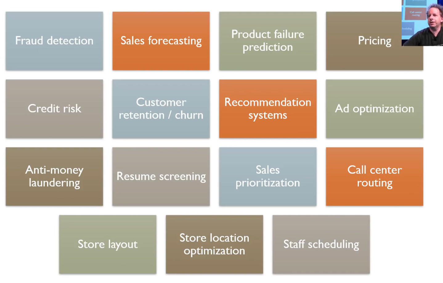
Using neural nets for analyzing tabular data is when we first presented this, people were deeply skeptical. They thought it was a terrible idea to use neural nets to analyze tabular data because everybody knows that you should use logistic regression, random forests, or gradient boosting machines (all of which have their place for certain types of things). But since that time, it’s become clear that the commonly held wisdom is wrong. It’s not true that neural nets are not useful for tabular data, in fact, they are extremely useful. We’ve shown this in quite a few of our courses, but what’s really helped is that some really effective organizations have started publishing papers and posts describing how they’ve been using neural nets for analyzing tabular data.
One of the key things that come up, again and again, is that although feature engineering doesn’t go away, it certainly becomes simpler. So Pinterest, for example, replaced the gradient boosting machines that they were using to decide how to put stuff on their homepage with neural nets. And they presented at a conference this approach, and they described how it really made engineering a lot easier because a lot of the hand created features weren’t necessary anymore. You still need some, but it was just simpler. So they ended up with something that was more accurate, but perhaps even more importantly, it required less maintenance. So Jeremy wouldn’t say you it’s the only tool that you need in your toolbox for analyzing tabular data. But where else, Jeremy used to use random forests 99% of the time when he was doing machine learning with tabular data, he now uses neural nets 90% of the time. It’s his standard first go-to approach now, and it tends to be pretty reliable and effective.
One of the things that’s made it difficult is that until now there hasn’t been an easy way to create and train tabular neural nets. Nobody has really made it available in a library. So we’ve actually just created fastai.tabular and I think this is pretty much the first time that’s become really easy to use neural nets with tabular data. So let me show you how easy it is.
Example [39:51]
This is actually coming directly from the examples folder in the fastai repo. Jeremy hasn’t changed it at all. As per usual, as well as importing fastai, import your application﹣so in this case, it’s tabular.
from fastai import *
from fastai.tabular import *
We assume that your data is in a Pandas DataFrame. Pandas DataFrame is the standard format for tabular data in Python. There are lots of ways to get it in there, but probably the most common might be pd.read_csv(). But whatever your data is in, you can probably get it into a Pandas dataframe easily enough.
path = untar_data(URLs.ADULT_SAMPLE)
df = pd.read_csv(path/'adult.csv')
Question: What are the 10% of cases where you would not default to neural nets?
[40:41]
Good question. Jeremy says he still tends to give them a try. But yeah, Jeremy doesn’t know. It’s kind of like as you do things for a while, you start to get a sense of the areas where things don’t quite work as well. Jeremy has to think about that during the week. Jeremy doesn’t think he has a rule of thumb. But he would say, you may as well try both. He would say try a random forest and try a neural net. They’re both pretty quick and easy to run, and see how it looks. If they’re roughly similar, Jeremy might dig into each and see if I can make them better. But if the random forest is doing way better, he’d probably just stick with that. Use whatever works.
So we start with the data in a data frame, and so we’ve got an adult sample﹣it’s a classic old dataset. It’s a pretty small simple old dataset that’s good for experimenting with. And it’s a CSV file, so you can read it into a data frame with Pandas read CSV (pd.read_csv()). If your data is in a relational database, Pandas can read from that. If it’s in spark or Hadoop, Pandas can read from that. Pandas can read from most stuff that you can throw at it. So that’s why we use it as a default starting point.
As per usual, I think it’s nice to use the data block API. So in this case, the list that we’re trying to create is a tabular list and we’re going to create it from a data frame.
test = TabularList.from_df(df.iloc[800:1000].copy(), path=path, cat_names=cat_names, cont_names=cont_names)
data = (TabularList.from_df(df, path=path, cat_names=cat_names, cont_names=cont_names, procs=procs)
                           .split_by_idx(list(range(800,1000)))
                           .label_from_df(cols=dep_var)
                           .add_test(test, label=0)
                           .databunch())
So you can tell it
- df - What the data frame is.
- path - What the path that you’re going to use to save models and intermediate steps are.
- cat_names, cont_names - you need to tell it what are your categorical variables and what are your continuous variables.
cat_names = ['workclass', 'education', 'marital-status', 'occupation', 'relationship', 'race']
cont_names = ['age', 'fnlwgt', 'education-num']
Continuous vs. Categorical Variables
We’re going to be learning a lot more about what that means to the neural net next week, but for now, the quick summary is this. Your independent variables are the things that you’re using to make predictions with. So things like education, marital status, age, and so forth.
Some of those variables like age are basically numbers. They could be any number.
You could be 13.36 years old or 19.4 years old or whatever.
Where else, things like marital status are options that can be selected from a discrete group: married, single, divorced, whatever.
Sometimes those options might be quite a lot more, like occupation. There’s a lot of possible occupations. And sometimes, they might be binary (i.e. true or false).
But anything which you can select the answer from a small group of possibilities is called a categorical variable. So we’re going to need to use a different approach in the neural net to modeling categorical variables to what we use for continuous variables.
For categorical variables, we’re going to be using something called embeddings which we’ll be learning about later today.
For continuous variables, they could just be sent into the neural net just like pixels in a neural net can. Because pixels in a neural net are already numbers; these continuous things are already numbers as well. So that’s easy.
So that’s why you have to tell the tabular list from data frame which ones are which. There are some other ways to do that by pre-processing them in Pandas to make things categorical variables, but it’s kind of nice to have one API for doing everything; you don’t have to think too much about it.
Processors (similar to transforms)
[45:04]
Then we’ve got something which is a lot like transforms in computer vision. Transforms in computer vision do things like flip a photo on its axis, turn it a bit, brighten it, or normalize it. But for tabular data, instead of having transforms, we have things called processors. And they’re nearly identical but the key difference, which is quite important, is that a processor is something that happens ahead of time. So we basically pre-process the data frame rather than doing it as we go. So transformations are really for data augmentation﹣we want to randomize it and do it differently each time. Or else, processors are the things that you want to do once, ahead of time.
procs = [FillMissing, Categorify, Normalize]
We have a number of processors in the fastai library. And the ones we’re going to use this time are -
- FillMissing: Look for missing values and deal with them some way.
- Categorify: Find categorical variables and turn them into Pandas categories
- Normalize: Do a normalization ahead of time which is to take continuous variables and subtract their mean and divide by their standard deviation so they are zero-one variables.
The way we deal with missing data, we’ll talk more about next week, but in short, we replace it with the median and add a new column which is a binary column of saying whether that was missing or not.
Normalization is an important thing here.
For all of these things, whatever you do to the training set, you need to do exactly the same thing to the validation set and the test set. So whatever you replaced your missing values with, you need to replace them with exactly the same thing in the validation set. So fastai handles all these details for you. They are the kinds of things that if you have to do it manually if you like Jeremy, you’ll screw it up lots of times until you finally get it right. So that’s what these processors are here.
data = (TabularList.from_df(df, path=path, cat_names=cat_names, cont_names=cont_names, procs=procs)
                           .split_by_idx(list(range(800,1000)))
                           .label_from_df(cols=dep_var)
                           .add_test(test, label=0)
                           .databunch())
-
split_by_idx() - Then we’re going to split into training versus validation sets. And in this case, we do it by providing a list of indexes so the indexes from 800 to a thousand. It’s very common. Jeremy doesn’t quite remember the details of this dataset, but it’s very common for wanting to keep your validation sets to be contiguous groups of things. If they’re map tiles, they should be the map tiles that are next to each other, if their time periods, they should be days that are next to each other, if they are video frames, they should be video frames next to each other. Because otherwise, you’re kind of cheating. So it’s often a good idea to use split_by_idx() and to grab a range that’s next to each other if your data has some kind of structure like that or find some other way to structure it in that way. All right, so that’s now given us training and a validation set.
-
label_from_df - We now need to add labels. In this case, the labels can come straight from the data frame we grabbed earlier, so we just have to tell it which column it is. So the dependent variable is whether they’re making over $50,000 salary. That’s the thing we’re trying to predict.
-
add_test() - We’ll talk about test sets later, but in this case, we can add a test set.
-
databunch() - And finally get our data bunch.
At that point, we have something that looks like this:
data.show_batch(rows=10)
| workclass | education | marital-status | occupation | relationship | race | education-num_na | age | fnlwgt | education-num | target |
|---|---|---|---|---|---|---|---|---|---|---|
| Private | 12th | Never-married | Other-service | Not-in-family | White | False | -1.2158 | 0.5291 | -0.8135 | 0 |
| Private | Some-college | Never-married | Exec-managerial | Not-in-family | Black | False | -1.0692 | 0.0235 | -0.0312 | 0 |
| Self-emp-not-inc | 1st-4th | Widowed | Other-service | Not-in-family | Black | False | 2.0826 | -0.7946 | -3.1604 | 0 |
| Private | Prof-school | Married-civ-spouse | Prof-specialty | Husband | White | False | -0.1896 | -0.3709 | 1.9245 | 0 |
There is our data. Then to use it, it looks very familiar. You get a learner, in this case, it’s a tabular learner, passing in the data, some information about your architecture(layers), and some metrics(accuracy). And you then call fit.
learn = tabular_learner(data, layers=[200,100], metrics=accuracy)

learn.fit(1, 1e-2)
Total time: 00:03
epoch  train_loss  valid_loss  accuracy
1      0.362837    0.413169    0.785000  (00:03)
Question: How to combine NLP (tokenized) data with metadata (tabular data) with Fastai? For instance, for IMBb classification, how to use information like who the actors are, year made, genre, etc.
[49:14]
Yeah, we’re not quite up to that yet. So we need to learn a little bit more about how neural net architectures work as well. But conceptually, it’s kind of the same as the way we combine categorical variables and continuous variables. Basically, in the neural network, you can have two different sets of inputs merging together into some layer. It could go into an early layer or into a later layer, it kind of depends. If it’s like text and an image and some metadata, you probably want the text going into an RNN, the image going into a CNN, the metadata going into some kind of tabular model like this. And then you’d have them basically all concatenated together, and then go through some fully connected layers and train them end to end. We will probably largely get into that in part two. In fact, we might entirely get into that in part two. I’m not sure if we have time to cover it in part one. But conceptually, it’s a fairly simple extension of what we’ll be learning in the next three weeks.
Question: Do you think that things like scikit-learn and xgboost will eventually become outdated? Will everyone will use deep learning tools in the future? Except for maybe small datasets?
[50:36]
Jeremy says he does not an idea. He’s not good at making predictions. He’s not a machine learning model. Jeremy means xgboost is a really nice piece of software. There’s quite a few really nice pieces of software for gradient boosting in particular. Actually, random forests, in particular, has some really nice features for interpretation which he’s sure we’ll find similar versions for neural nets, but they don’t necessarily exist yet. So he doesn’t know. For now, they’re both useful tools. scikit-learn is a library that’s often used for pre-processing and running models. Again, it’s hard to predict where things will end up. In some ways, it’s more focused on some older approaches to modeling, but he doesn’t know. They keep on adding new things, so we’ll see. He keeps trying to incorporate more scikit-learn stuff into fastai and then he keeps finding ways he thinks he can do it better and he throws it away again, so that’s why there’s still no scikit-learn dependencies in fastai. He keeps finding other ways to do stuff.
Tabular learner[52:12]
layers=[200,100]
We’re gonna learn what layers means either towards the end of class today or the start of class next week, but this is where we’re basically defining our architecture just like when we chose ResNet 34 or whatever for convolutional neural networks. We’ll look at more about metrics in a moment, but just to remind you, metrics are just the things that get printed out. They don’t change our model at all. So in this case, we’re saying we want you to print out the accuracy to see how we’re doing.
So that’s how to do tabular. This is going to work really well because we’re gonna hit our break soon. And the idea was that after three and a half lessons, we’re going to hit the end of all of the quick overview of applications, and then I’m going to go down on the other side. I think we’re going to be to the minute, we’re going to hit it. Because the next one is collaborative filtering.
Collaborative Filtering[53:08]
Collaborative filtering is where you have information about who bought what, or who liked what﹣ it’s basically something where you have something like a user, a reviewer, or whatever and information about what they’ve bought, what they’ve written about, or what they reviewed. So in the most basic version of collaborative filtering, you just have two columns: something like user ID and movie ID and that just says this user bought that movie. So for example, Amazon has a really big list of user IDs and product IDs like what did you buy. Then you can add additional information to that table such as oh, they left a review, what review did they give it? So it’s now like user ID, movie ID, number of stars. You could add a timecode so this user bought this product at this time and gave it this review. But they are all basically the same structure.
There are two ways you could draw that collaborative filtering structure. One is a two-column approach where you’ve got user and movie. And you’ve got the user ID, movie ID﹣each pair basically describes that user watches that movie, possibly also the number of stars (3, 4, etc). The other way you could write it would be you could have like all the users down here and all the movies along here. And then, you can look and find a particular cell in there to find out what could be the rating of that user for that movie, or there’s just a 1 there if that user watched that movie, or whatever.
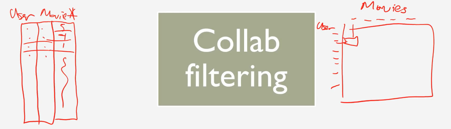
So there are two different ways of representing the same information. Conceptually, it’s often easier to think of it this way (the format on the right), but most of the time you won’t store it that way. Explicitly because most of the time, you’ll have what’s called a very sparse matrix which is to say most users haven’t watched most movies or most customers haven’t purchased most products. So if you store it as a matrix where every combination of customer and product is a separate cell in that matrix, it’s going to be enormous. So you tend to store it like the left or you can store it as a matrix using some kind of special sparse matrix format. If that sounds interesting, you should check out Rachel’s computational linear algebra course on fastai where we have lots and lots of information about sparse matrix storage approaches. For now though, we’re just going to kind of keep it in this format on left hand side.
Movielens Example [56:38]
For collaborative filtering, there’s a really nice dataset called MovieLens created by GroupLens group and you can download various different sizes (20 million ratings, 100,000 ratings). We’ve actually created an extra small version for playing around with which is what we’ll start with today. And then probably next week, we’ll use the bigger version.
from fastai import *
from fastai.collab import *
from fastai.tabular import *
You can grab the small version using URLs.ML_SAMPLE:
user,item,title = 'userId','movieId','title'
path = untar_data(URLs.ML_SAMPLE)
path
PosixPath('/home/jhoward/.fastai/data/movie_lens_sample')
ratings = pd.read_csv(path/'ratings.csv')
ratings.head()
It’s a CSV so you can read it with Pandas and here it is. It’s basically a list of user IDs﹣we don’t actually know anything about who these users are. There are some movie IDs. There is some information about what the movies are, but we won’t look at that until next week. Then there’s the rating and the timestamp. We’re going to ignore the timestamp for now. So that’s a subset of our data.head() in Pandas is just the first few rows.
So now that we’ve got a data frame, the nice thing about collaborative filtering is it’s incredibly simple.
data = CollabDataBunch.from_df(ratings, seed=42)
y_range = [0,5.5]
learn = collab_learner(data, n_factors=50, y_range=y_range)
That’s all the data that we need. So you can now go ahead and say get collab_learner() and you can pass in the data bunch(data).
- n_factors - The architecture, you have to tell it how many factors(n_factors) you want to use, and we’re going to learn what that means after the break.
- y_range - And then something that could be helpful is to tell it what the range of scores are. We’re going to see how that helps after the break as well. So in this case, the minimum score is 0, the maximum score is 5.
learn.fit_one_cycle(3, 5e-3)
Total time: 00:04
epoch  train_loss  valid_loss
1      1.600185    0.962681    (00:01)
2      0.851333    0.678732    (00:01)
3      0.660136    0.666290    (00:01)
Now that you’ve got a learner, you can go ahead and call fit_one_cycle and trains for a few epochs, and there it is. So at the end of it, you now have something where you can pick a user ID and a movie ID, and guess whether or not that user will like that movie.
Cold start problem [58:53]
This is obviously a super useful application that a lot of you are probably going to try during the week. In past classes, a lot of people have taken this collaborative filtering approach back to their workplaces and discovered that using it in practice is much more tricky than this. Because in practice, you have something called the cold start problem. So the cold start problem is that the time you particularly want to be good at recommending movies is when you have a new user, and the time you particularly care about recommending a movie is when it’s a new movie. But at that point, you don’t have any data in your collaborative filtering system and it’s really hard.
As Jeremy says this, we don’t currently have anything built into fastai to handle the cold start problem and that’s really because the cold start problem, the only way Jeremy know of to solve it (in fact, the only way Jeremy thinks that conceptually can solve it) is to have a second model which is not a collaborative filtering model but a metadata-driven model for new users or new movies.
Jeremy doesn’t know if Netflix still does this, but certainly what they used to do when Jeremy signed up to Netflix was they started showing me lots of movies and saying “have you seen this?” “did you like it?” ﹣so they fixed the cold start problem through the UX, so there was no cold start problem. They found like 20 really common movies and asked me if Jeremy liked them, they used his replies to those 20 to show me 20 more that Jeremy might have seen, and by the time he had gone through 60, there was no cold start problem anymore.
For new movies, it’s not really a problem because like the first hundred users who haven’t seen the movie go in and say whether they liked it, and then the next hundred thousand, the next million, it’s not a cold start problem anymore.
The other thing you can do if you, for whatever reason, can’t go through that UX of asking people did you like those things (for example if you’re selling products and you don’t really want to show them a big selection of your products and say did you like this because you just want them to buy), you can instead try and use a metadata-based tabular model what geography did they come from maybe you know their age and sex, you can try and make some guesses about the initial recommendations.
So collaborative filtering is specifically for once you have a bit of information about your users and movies or customers and products or whatever.
[1:01:36]
Question: How does the language model trained in this manner perform on code switched data (Hindi written in English words), or text with a lot of emojis?
Text with emojis, it’ll be fine. There are not many emojis in Wikipedia and where they are at Wikipedia it’s more like a Wikipedia page about the emoji rather than the emoji being used in a sensible place. But you can (and should) do this language model fine-tuning where you take a corpus of text where people are using emojis in usual ways, and so you fine-tune the Wikitext language model to your Reddit or Twitter or whatever language model. And there aren’t that many emojis if you think about it. There are hundreds of thousands of possible words that people can be used, but a small number of possible emojis. So it’ll very quickly learn how those emojis are being used. So that’s a piece of cake.
I’m not really familiar with Hindi, but I’ll take an example I’m very familiar with which is Mandarin. In Mandarin, you could have a model that’s trained with Chinese characters. There are about five or six thousand Chinese characters in common use, but there’s also a romanization of those characters called pinyin. It’s a bit tricky because although there’s a nearly direct mapping from the character to the pinyin (I mean there is a direct mapping but that pronunciations are not exactly direct), there isn’t direct mapping from the pinyin to the character because one pinyin corresponds to multiple characters.
So the first thing to note is that if you’re going to use this approach for Chinese, you would need to start with a Chinese language model.
Actually, fastai has something called Language Model Zoo where we’re adding more and more language models for different languages, and also increasingly for different domain areas like English medical texts or even language models for things other than NLP like genome sequences, molecular data, musical MIDI notes, and so forth. So you would you obviously start there.
To then convert that (in either simplified or traditional Chinese) into pinyin, you could either map the vocab directly, or as you’ll learn, these multi-layer models﹣it’s only the first layer that basically converts the tokens into a set of vectors, you can actually throw that away and fine-tune just the first layer of the model. So that second part is going to require a few more weeks of learning before you exactly understand how to do that and so forth, but if this is something you’re interested in doing, we can talk about it on the forum because it’s a nice test of understanding.
Question: What about time series on tabular data? is there any RNN model involved in tabular.models?
[1:05:09]
We’re going to look at time series tabular data next week, but the short answer is generally speaking you don’t use an RNN for time series tabular data but instead, you extract a bunch of columns for things like day of week, is it a weekend, is it a holiday, was the store open, stuff like that. It turns out that adding those extra columns which you can do somewhat automatically basically gives you state-of-the-art results. There are some good uses of RNNs for time series, but not really for these kinds of tabular style time series (like retail store logistics databases, etc).
Question: Is there a source to learn more about the cold start problem?
[1:06:14]
I’m gonna have to look that up. If you know a good resource, please mention it on the forums.
The halfway point [1:06:34]
[1:06:34]
That is both the break in the middle of lesson 4, it’s the halfway point of the course, and it’s the point at which we have now seen an example of all the key applications. So the rest of this course is going to be digging deeper into how they actually work behind the scenes, more of the theory, more of how the source code is written, and so forth. So it’s a good time to have a nice break. Furthermore, it’s Jeremy’s birthday today, so it’s a really special moment.
Collaborative filtering with Microsoft Excel
[1:07:25]
Microsoft Excel is one of Jeremy’s favorite ways to explore data and understand models. Actually this one, we can probably largely do in Google Sheets. Jeremy has tried to move as much as he can over the last few weeks into Google Sheets, but I just keep finding this is such a terrible product, so please try to find a copy of Microsoft Excel because there’s nothing close, I’ve tried everything. Anyway, spreadsheets get a bad rap from people that basically don’t know how to use them. Just like people who spend their life on Excel and then they start using Python, and they’re like what the heck is this stupid thing. It takes thousands of hours to get really good at spreadsheets, but a few dozen hours to get confident at them. Once you’re confident at them, you can see everything in front of you. It’s all laid out, it’s really great.
Jeremy’s spreadsheet tip of the day.
[1:08:37]
Jeremy is giving you one spreadsheet tip today which is if you hold down the
control key or command key
and press the arrow keys, here’s control + →
, it takes you to the end of a block of a table that you’re in. And it’s by far the best way to move around the place, so there you go.
In this case, we want to skip around through this table, so we can hit control+ ↓ +→ to get to the bottom right, ctrl+ ←+ ↑ to get to the top left. Skip around and see what’s going on.
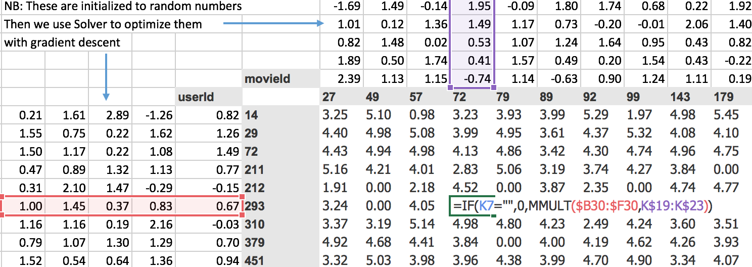
So here’s some data, and as we talked about, one way to look at collaborative filtering data is like this
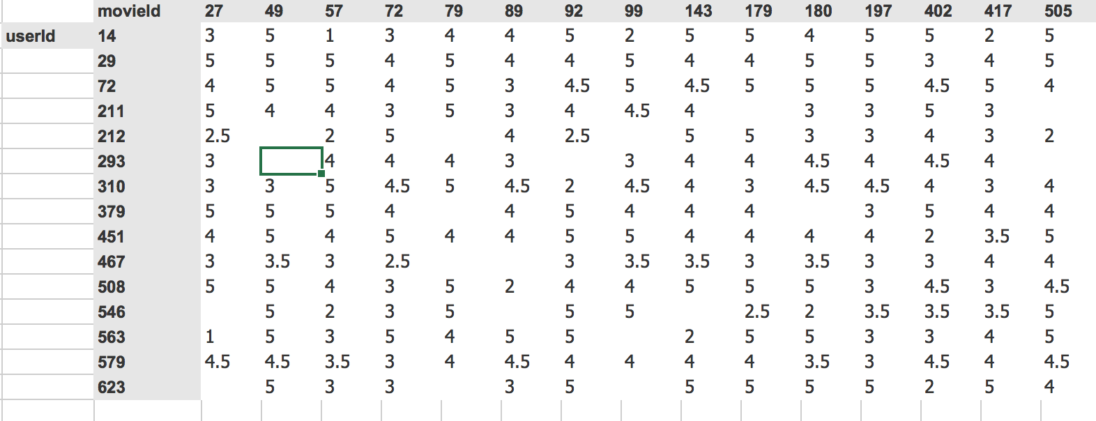
What we did was we grabbed from the MovieLens data the people that watched the most movies and the movies that were the most watched and just filtered the dataset down to those 15. As you can see, when you do it that way, it’s not sparse anymore. There’s just a small number of gaps.
This is something that we can now build a model with. How can we build a model? What we want to do is we want to create something which can predict for user 293, will they like movie 49, for example. So we’ve got to come up with some function that can represent that decision.
Here’s a simple possible approach. We’re going to take this idea of doing some matrix multiplications. So I’ve created here a random matrix. So here’s one matrix of random numbers (the left). And I’ve created here another matrix of random numbers (the top). More specifically, for each movie, I’ve created five random numbers, and for each user, I’ve created five random numbers.
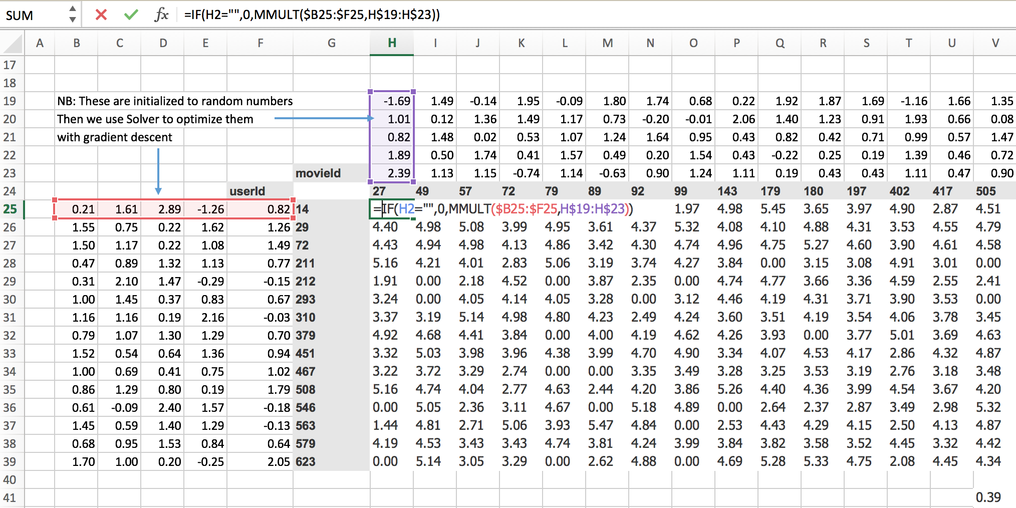
So we could say, then, that user 14, movie 27; did they like it or not? Well, the rating, what we could do would be to multiply together this vector (red) and that vector (purple). We could do a dot product, and here’s the dot product. Then we can basically do that for every possible thing in here. And thanks to spreadsheets, we can just do that in one place and copy it over, and it fills in the whole thing for us. Why would we do it this way? Well, this is the basic starting point of a neural net, isn’t it? A basic starting point of a neural net is that you take the matrix multiplication of two matrices, and that’s what your first layer always is. So we just have to come up with some way of saying what are two matrices that we can multiply. Clearly, you need a vector for a user (a matrix for all the users) and a vector for a movie (a matrix for all the movies) and multiply them together, and you get some numbers. So they don’t mean anything yet. They’re just random. But we can now use gradient descent to try to make these numbers (top) and these numbers (left) give us results that are closer to what we wanted.
So how do we do that? Well, we set this up now as a linear model, so the next thing we need is a loss function. We can calculate our loss function by saying well okay movie 27 for user ID 14 should have been a rating of 3. With this random matrices, it’s actually a rating of 0.91, so we can find the sum of squared errors would be (3-0.91)2
and then we can add them up. So there’s actually a sum squared in Excel already sum X minus y squared ( SUMXMY2), so we can use just sum X minus y squared function, passing in those two ranges and then divide by the count to get the mean.
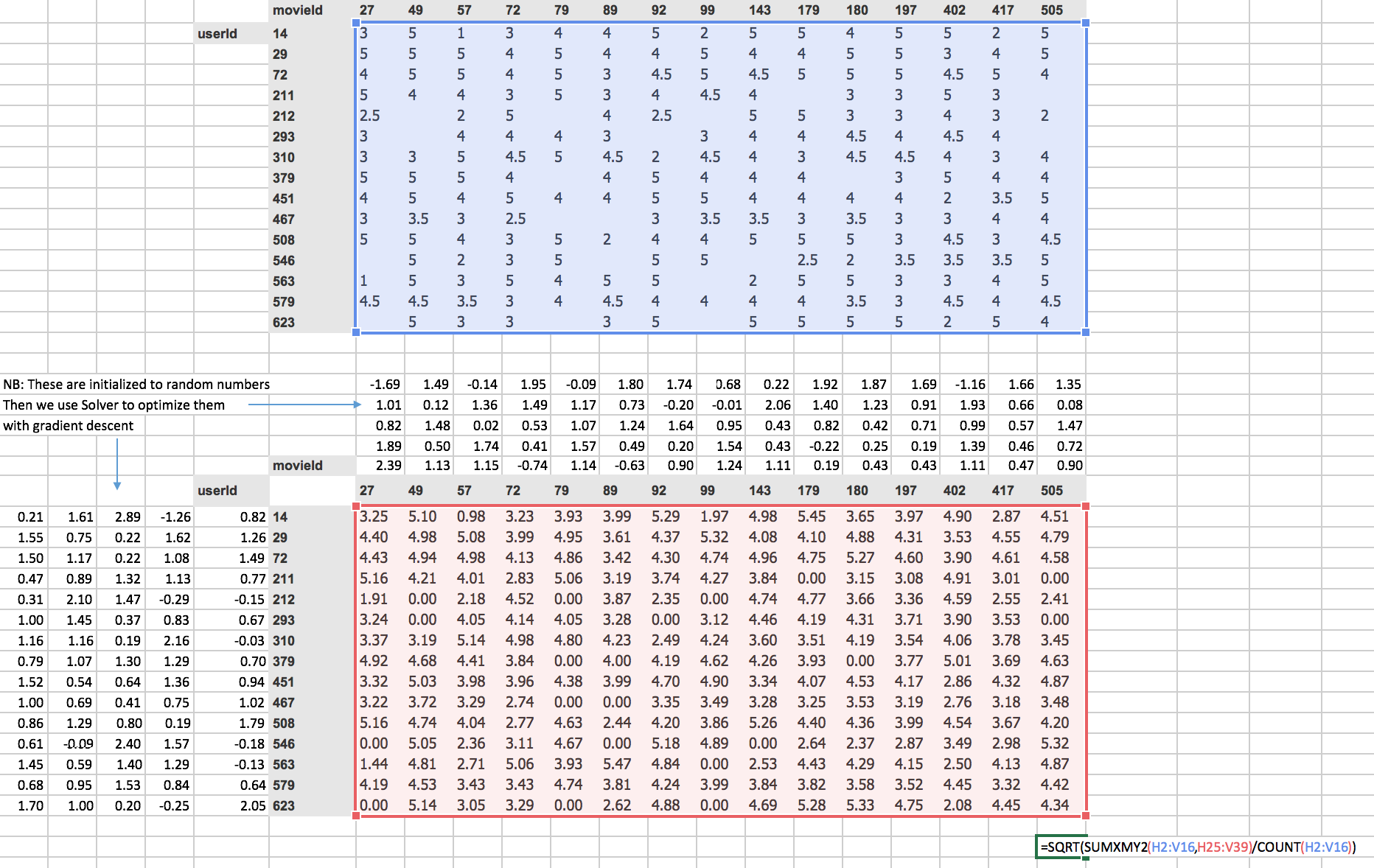
Here is a number that is the square root of the mean squared error. You sometimes you’ll see people talk about MSE so that’s the Mean Squared Error, sometimes you’ll see RMSE that’s the Root Mean Squared Error. Since we’ve got a square root at the front, this is the square root mean square error.
Excel Solver
[1:14:30]
We have a loss, so now all we need to do is use gradient descent to try to modify our weight matrices to make that loss smaller. Excel will do that for us.
If you don’t have solver, go to Excel Options → Add-ins, and enable Solver Add-in.
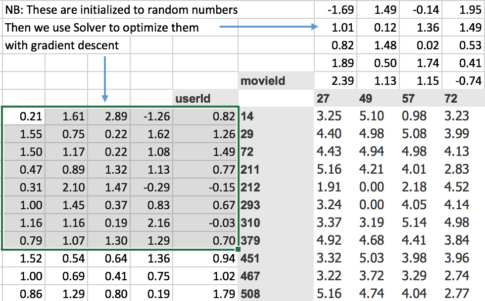
The gradient descent solver in Excel is called “Solver” and it just does normal gradient descent. You just go Data → Solver (you need to make sure that in your settings that you’ve enabled the solver extension which comes with Excel) and all you need to do is say which cell represents our loss function. So there it is, cell V41. Which cells contain your variables, and so you can see here, we’ve got H19 to V23 which is up here, and B25 to F39 which is over there, then you can just say “okay, set your loss function to a minimum by changing those cells” and click on Solve.
You’ll see the starts a 2.81, and you can see the numbers going down. And all that’s doing is using gradient descent exactly the same way that we did when we did it manually in the notebook the other day. But it’s rather than solving the mean squared error for a@x in Python, instead, it is solving the loss function here which is the mean squared error of the dot product of each of those vectors by each of these vectors.
We’ll let that run for a little while and see what happens. But basically in micro, here is a simple way of creating a neural network which is really in this case, it’s like just a single linear layer with gradient descent to solve a collaborative filtering problem.
The collab filter notebook
[1:17:03]
Let’s go back and see what we do over here.
data = CollabDataBunch.from_df(ratings, seed=42)
y_range = [0,5.5]
learn = collab_learner(data, n_factors=50, y_range=y_range)
learn.fit_one_cycle(3, 5e-3)
Total time: 00:04
epoch  train_loss  valid_loss
1      1.600185    0.962681    (00:01)
2      0.851333    0.678732    (00:01)
3      0.660136    0.666290    (00:01)
So over here we used collab_learner to get a model. So the function that was called in the notebook was collab_learner and as you dig deeper into deep learning, one of the really good ways to dig deeper into deep learning is to dig into the fastai source code and see what’s going on. So if you’re going to be able to do that, you need to know how to use your editor well enough to dig through the source code. Basically, there are two main things you need to know how to do
- Jump to a particular “symbol”, like a particular class or function by its name
- When you’re looking at a particular symbol, to be able to jump to its implementation
For example, in this case, I want to find def collab_learner(). In most editors including the one I use, vim, you can set it up so that you can hit tab or something and it jumps through all the possible completions, and you can hit enter and it jumps straight to the definition for you. So here is the definition of collab_learner.
def collab_learner(data, n_factors:int=None, use_nn:bool=False, metrics=None,
                   emb_szs:Dict[str,int]=None, wd:float=0.01, **kwargs)->Learner:
    "Create a Learner for collaborative filtering on `data`."
    emb_szs = data.get_emb_szs(ifnone(emb_szs, {}))
    u,m = data.classes.values()
    if use_nn: model = EmbeddingNN(emb_szs=emb_szs, **kwargs)
    else:      model = EmbeddingDotBias(n_factors, len(u), len(m), **kwargs)
    return CollabLearner(data, model, metrics=metrics, wd=wd)
As you can see, it’s pretty small as these things tend to be, and the key thing it does is to create the model of a particular kind which is an EmbeddingDotBias model passing in the various things you asked for. So you want to find out in your editor how you jump to the definition of that, which in vim you just hit control+ [and here is the definition of EmbeddingDotBias.
class EmbeddingDotBias(nn.Module):
    "Base dot model for collaborative filtering."
    def __init__(self, n_factors:int, n_users:int, n_items:int, y_range:Tuple[float,float]=None):
        super().__init__()
        self.y_range = y_range
        (self.u_weight, self.i_weight, self.u_bias, self.i_bias) = [embedding(*o) for o in [
            (n_users, n_factors), (n_items, n_factors), (n_users,1), (n_items,1)
        ]]

    def forward(self, users:LongTensor, items:LongTensor) -> Tensor:
        dot = self.u_weight(users)* self.i_weight(items)
        res = dot.sum(1) + self.u_bias(users).squeeze() + self.i_bias(items).squeeze()
        if self.y_range is None: return res
        return torch.sigmoid(res) * (self.y_range[1]-self.y_range[0]) + self.y_range[0]
Now we have everything on screen at once, and as you can see there’s not much going on. The models that are being created for you by fastai are actually PyTorch models. And a PyTorch model is called an nn.Module that’s the name in PyTorch of their models. It’s a little more nuanced than that, but that’s a good starting point for now. When a PyTorch nn.Module is run (when you calculate the result of that layer, neural net, etc), specifically, it always calls a method for you called forward(). So it’s in here that you get to find out how this thing is actually calculated.
When the model is built at the start, it calls this thing called _ _ init _ _() as we’ve briefly mentioned before in Python people tend to call these methods which start and end with double underscores as dunder methods. So _ _ init _ _()(dunder init, note while writing there is no space between underscores in code) is how we create the model, and forward() is how we run the model.
One thing if you’re watching carefully, you might notice is there’s nothing here saying how to calculate the gradients of the model, and that’s because PyTorch does it for us. So you only have to tell it how to calculate the output of your model, and PyTorch will go ahead and calculate the gradients for you.
So in this case, the model contains:
- a set of weights for a user - self.u_weight
- a set of weights for an item - self.i_weight
- a set of biases for a user - self.u_bias
- a set of biases for an item - self.i_bias
Embeddings
And each one of those is coming from this method called embedding(). Here is the definition of embedding
def embedding(ni:int,nf:int) -> nn.Module:
    "Create an embedding layer."
    emb = nn.Embedding(ni, nf)
    # See https://arxiv.org/abs/1711.09160
    with torch.no_grad(): trunc_normal_(emb.weight, std=0.01)
    return emb
All it does is it calls this PyTorch thing called nn.Embedding. In PyTorch, they have a lot of standard neural network layers set up for you. So it creates an embedding. And then this thing here (trunc_normal_) is it just randomizes it. This is something which creates normal random numbers for the embedding.
So what’s an embedding? An embedding, not surprisingly, is a matrix of weights. Specifically, an embedding is a matrix of weights that looks something like this.
It’s a matrix of weights which you can basically look up into, and grab one item out of it. So basically an embedding matrix is just a weight matrix that is designed to be something that you index into it as an array, and grab one vector out of it. That’s what an embedding matrix is. In our case, we have an embedding matrix for a user and an embedding matrix for a movie. And here, we have been taking the dot product of them:
But if you think about it, that’s not quite enough. Because we’re missing this idea that maybe there are certain movies that everybody likes more. Maybe there are some users that just tend to like movies more. So I don’t really just want to multiply these two vectors together, but I really want to add a single number of like how popular is this movie, and add a single number of like how much does this user like movies in general. So those are called “bias” terms. Remember how I said there’s this idea of bias and the way we dealt with that in our gradient descent notebook was we added a column of 1’s. But what we tend to do in practice is we actually explicitly say I want to add a bias term. So we don’t just want to have prediction equals dot product of these two things, we want to say it’s the dot product of those two things plus a bias term for a movie plus a bias term for the user ID.
Back to code
[1:23:50]
So that’s basically what happens. We when we set up the model, we set up the embedding matrix for the users and the embedding matrix for the items. And then we also set up the bias vector for the users and the bias vector for the items.
Then when we calculate the model, we literally just multiply the two together. Just like we did. We just take that product, we call it dot product. Then we add the bias, and (putting aside y_range for a moment) that’s what we return. So you can see that our model is literally doing what we did in the spreadsheet with the tweak that we’re also adding the bias. So it’s an incredibly simple linear model. For these kinds of collaborative filtering problems, this kind of simple linear model actually tends to work pretty well.
Then there’s one tweak that we do at the end which is that in our case we said that there’s y range of between 0 and 5.5. So here’s something to point out. So you do that dot product and you add on the two biases and that could give you any possible number along with the number line from very negative through to very positive numbers. But we know that we always want to end up with a number between zero and five. What if we mapped that number line like so, to this function. The shape of that function is called a sigmoid. And so, it’s gonna asymptote to five and it’s gonna asymptote to zero.
That way, whatever number comes out of our dot product and adding the biases, if we then stick it through this function, it’s never going to be higher than 5 and never going to be smaller than 0. Now, strictly speaking, that’s not necessary. Because our parameters could learn a set of weights that gives about the right number. So why would we do this extra thing if it’s not necessary? The reason is, we want to make its life as easy for our model as possible. If we actually set it up so it’s impossible for it to ever predict too much or too little, then it can spend more of its weights predicting the thing we care about which is deciding who’s going to like which movie. So this is an idea we’re going to keep coming back to when it comes to like making neural network’s work better. It’s about all these little decisions that we make to basically make it easier for the network to learn the right thing. So that’s the last tweak here:
return torch.sigmoid(res) * (self.y_range[1]-self.y_range[0]) + self.y_range[0]
We take the result of this dot product plus biases, we put it through a sigmoid. A sigmoid is just a function which is basically
\frac{1}{1+e^{-x}}
but the definition doesn’t much matter. But it just has the shape that I just mentioned, and that goes between 0 and 1. If you then multiply that by y_range[1] minus y_range[0] plus y_range[0], then that’s going to give you something that’s between y_range[0] and y_range[1].
So that means that this tiny little neural network, I mean it’s a push to call it a neural network. But it is a neural network with one weight matrix and no nonlinearities. So it’s kind of the world’s most boring neural network with a sigmoid at the end. I guess it does have a non-linearity. The sigmoid at the end is the non-linearity, it only has one layer of weights. That actually turns out to give close to the state-of-the-art performance. I’ve looked up online to find out like what are the best results people have on this MovieLens 100k database, and the results I get from this little thing is better than any of the results I can find from the standard commercial products that you can download that are specialized for this. And the trick seems to be that adding this little sigmoid makes a big difference.
Question: There was a question about how you set up your vim, and we’ve already linked to your .vimrc but we wanted to know if you had more to say about. They really like your setup 
[1:29:10]
Do you like Jeremy’s setup? There’s almost nothing in his setup. It’s pretty bare honestly. I mean whatever you’re doing with your editor, you probably want it to look like this which is when you’ve got a class that you’re not currently working on it should be this is called folded/folding﹣it should be closed up so you can’t see it. So you basically want something where it’s easy to close and open folds, so vim already does all this for you. Then as I mentioned, you also want something where you can jump to the definition of things which in vim called using tags (e.g. to jump to the definition of Learner, position the cursor over Learner and hit Ctrl+]). Basically, vim already does all this for you. You just have to read instructions. My .vimrc is minimal. I basically hardly use any extensions or anything. Another great editor to use is a Visual Studio Code. It’s free and it’s awesome and it has all the same features that you’re seeing that vim does, basically, VS Sode does all of those things as well. Jeremy quite likes using vim because he can use it on the remote machine and play around, but you can of course just clone the git repo into your local computer and open it up with VS Code to play around with. Just don’t try and look through the code just on GitHub or something. That’s going to drive you crazy. You need to be able to open it and close it and jump and jump back. Maybe people can create some threads on the forum for vim tips, VS Code tips, Sublime tips, whatever. For me, I would if you’re gonna pick an editor, if you want to use something on your local, he would go with the VS Code today. He thinks it’s the best. If you want to use something on the terminal side, Jeremy would go with VIM or Emacs, to him they’re clear winners.
Overview of important terminology [1:31:24]
So what Jeremy wanted to close with today is, to take this collaborative filtering example and describe how we’re going to build on top of it for the next three lessons to create the more complex neural networks we’ve been seeing. Roughly speaking, this is the bunch of concepts that we need to learn about -
- Inputs
- Weights/parameters
- Random
- Activations
- Activation functions / nonlinearities
- Output
- Loss
- Metric
- Cross-entropy
- Softmax
- Fine tuning
- Layer deletion and random weights
- Freezing & unfreezing
Let’s think about what happens when you’re using a neural network to do image recognition. Let’s take a single pixel. You’ve got lots of pixels, but let’s take a single pixel. So you’ve got a red a green and a blue pixel. Each one of those is some number between 0 and 255, or we normalize them so they have the mean of zero and standard deviation of one. But let’s just do 0 to 255 version. So red: 10, green: 20, blue 30. So what do we do with these? Well, what we do is we basically treat that as a vector, and we multiply it by a matrix. So this matrix (depending on how you think of the rows and the columns), let’s treat the matrix is having three rows and then how many columns? You get to pick. Just like with the collaborative filtering version, I decided to pick a vector of size five for each of my embedding vectors. So that would mean that’s an embedding of size 5. You get to pick how big your weight matrix is. So let’s make it size 5. This is 3 by 5.
Initially, this weight matrix contains random numbers. Remember we looked at embedding weight matrix just now?
def embedding(ni:int,nf:int) -> nn.Module:
    "Create an embedding layer."
    emb = nn.Embedding(ni, nf)
    # See https://arxiv.org/abs/1711.09160
    with torch.no_grad(): trunc_normal_(emb.weight, std=0.01)
    return emb
There were two lines; the first line created the matrix, and the second was fill it with random numbers? That’s all we do. It all gets hidden behind the scenes by fastai and PyTorch, but that’s all it’s doing. So it’s creating a matrix of random numbers when you set it up. The number of rows has to be 3 to match the input, and the number of columns can be as big as you like. So after you multiply the input vector by that weight matrix, you’re going to end up with a vector of size 5.
People often ask how much linear algebra do I need to know to be able to do deep learning. This is the amount you need. And if you’re not familiar with this, that’s fine. You need to know about matrix products. You don’t need to know a lot about them, you just need to know like computationally what are they and what do they do. You’ve got to be very comfortable with if a matrix of size blah times a matrix of size blah gives a matrix or size blah (i.e. how do the dimensions match up). So if you have 3, and they remember in numpy and PyTorch, we use @ times 3 by 5 gives a vector of size 5.
Then what happens next; it goes through an activation function such as ReLU which is just max(0,x) and spits out a new vector which is, of course, going to be exactly the same size because no activation function changes the size﹣it only changes the contents. So that’s still of size 5.
What happens next? We multiply by another matrix. Again, it can be any number of columns, but the number of rows has to map nicely. So it’s going to be 5 by whatever. Maybe this one has 5, let’s say, by 10. That’s going to give some output﹣it should be size 10 and again we put that through ReLU, and again that gives us something of the same size.
Then we can put that through another matrix. Actually, just to make this a bit clearer (you’ll see why in a moment), Jeremy is going to use 8, not 10.
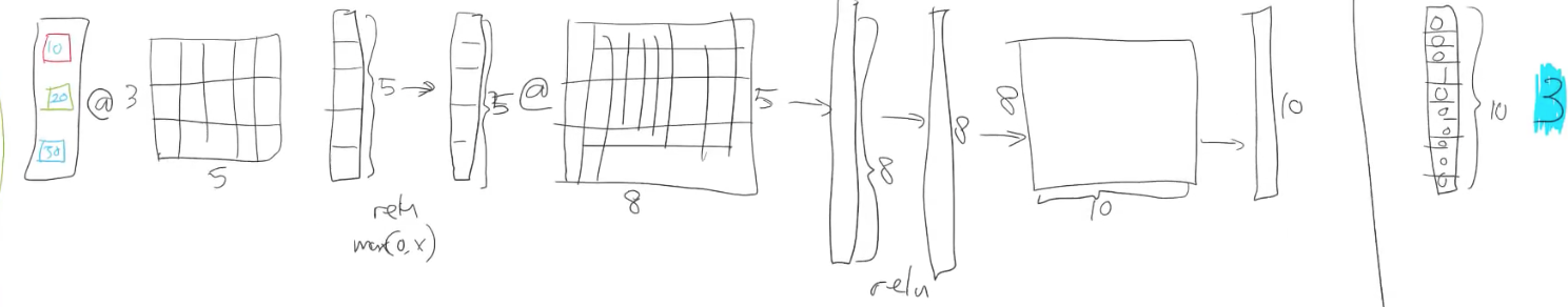
Let’s say we’re doing digit recognition. There are ten possible digits, so my last weight matrix has to be 10 in size. Because then that’s going to mean my final output is a vector of 10 in size. Remember if you’re doing that digit recognition, we take our actuals which are 10 in size. And if the number we’re trying to predict was the number 3, then that means that there is a 1 in the third position ([0,0,0,1,0,…]).
So what happens is our neural net runs along starting with our input, and going weight matrix→ReLU→ weight matrix→ReLU→ weight matrix→ final output. Then we compare these two together to see how close they are (i.e. how close they match) using some loss function and we’ll learn about all the loss functions that we use next week. For now, the only one we’ve learned is mean squared error. And we compare the output (you can think of them as probabilities for each of the 10) to the actual each of the 10 to get a loss, and then we find the gradients of every one of the weight matrices with respect to that, and we update the weight matrices.
The main thing Jeremy wanted to show right now is the terminology we use because it’s really important.
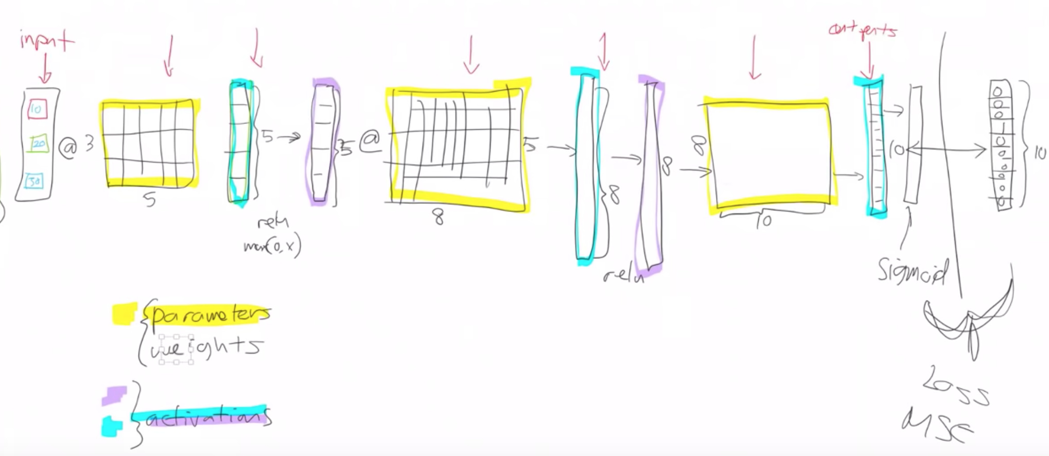
These things (yellow) contain numbers. Specifically, they initially are matrices containing random numbers. And we can refer to these yellow things, in PyTorch, they’re called parameters. Sometimes we’ll refer to them as weights, although weights are slightly less accurate because they can also be biased. But we kind of use the terms a little bit interchangeably. Strictly speaking, we should call them parameters.
Then after each of those matrix products, that calculates a vector of numbers. Here are some numbers (blue) that are calculated by a weight matrix multiply. And then there’s some other set of numbers (purple) that are calculated as a result of a ReLU as well as the activation function. Either one is called activations.
Activations and parameters, both refer to numbers. They are numbers. But Parameters are numbers that are stored, they are used to make a calculation. Activations are the result of a calculation﹣the numbers that are calculated. So they’re the two key things you need to remember.
So use these terms, and use them correctly and accurately. And if you read these terms, they mean these very specific things. So don’t mix them up in your head. And remember, they’re nothing weird and magical﹣they are very simple things.
An activation is the result of either a matrix multiply or an activation function.
Parameters are the numbers inside the matrices that we multiply by.
That’s it. Then there are some special layers. Every one of these things that does a calculation, all of these things that does a calculation (red arrow), are all called layers. They’re the layers of our neural net. So every layer results in a set of activations because there’s a calculation that results in a set of results.
There’s a special layer at the start which is called the input layer, and then at the end, you just have a set of activations and we can refer to those special numbers (I mean they’re not special mathematically but they’re semantically special); we can call those the outputs. The important point to realize here is the outputs of a neural net are not actually mathematically special, they’re just the activations of a layer.
So what we did in our collaborative filtering example, we did something interesting. We actually added an additional activation function right at the very end. We added an extra activation function which was sigmoid, specifically it was a scaled sigmoid which goes between 0 and 5. It’s very common to have an activation function as your last layer, and it’s almost never going to be a ReLU because it’s very unlikely that what you actually want is something that truncates at zero. It’s very often going to be a sigmoid or something similar because it’s very likely that actually what you want is something that’s between two values and kind of scale in that way.
So that’s nearly it. Inputs, weights, activations, activation functions (which we sometimes call nonlinearities), output, and then the function that compares those two things together is called the loss function, which so far we’ve used MSE.
That’s enough for today. So what we’re going to do next week is we’re going to kind of add in a few more extra bits which is we’re going to learn the loss function that’s used for classification called cross-entropy, we’re going to use the activation function that’s used for single-label classification called softmax, and we’re also going to learn exactly what happens when we do fine-tune in terms of how these layers actually, what happens with unfreeze, and what happens when we create transfer learning. Thanks, everybody! Looking forward to seeing you next week.
