This is a forum wiki thread, so you all can edit this post to add/change/ organize info to help make it better! To edit, click on the little pencil icon at the bottom of this post. Here’s a pic of what to look for:
![]()
<<< Notes: Lesson 2 | Notes: Lesson 4 >>>
Thanks, Jeremy for another great lecture.
Hi everybody, welcome to lesson 3.
Multi-label, Segmentation, Image Regression, and More…
Important posts to watch:
Software Update
![]() Always remember to do an update on the fast.ai library and course repo.
Always remember to do an update on the fast.ai library and course repo.
conda install -c fastai fastai for the library update
git pull for the course repo update.
Lesson 3 Notebooks:
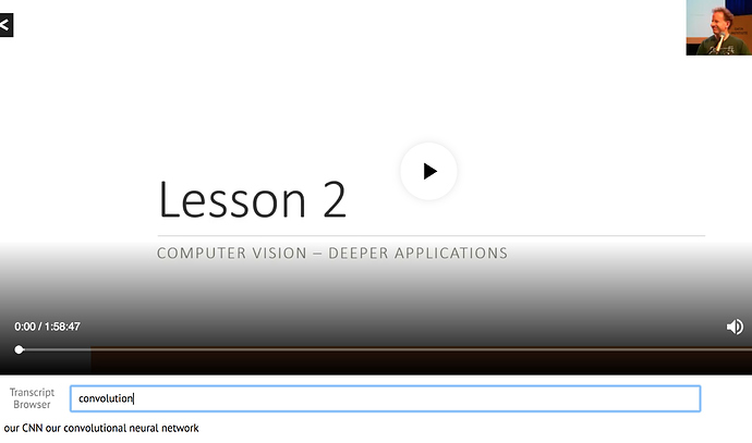
Video Browser with Searchable Transcripts
This week one student Zack from San Fransisco Study group created a video player for lessons.
Video Browser with Searchable Transcripts
Password: deeplearningSF2018 (do not share outside the forum group)
You can search text in the transcript browser. It will give you a link to jump on that part of the video.
The transcript right now is not great since it’s coming from google auto transcript.
The next step is to use a neural network to get a better transcript.
If you want to help in that please free to join us even if you are not in San Francisco.
Correction [00:06]
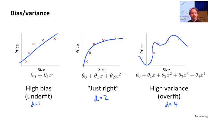
There is a correction. Jeremy mentioned in the previous lecture that the diagram below was from a Quora thread. But it’s from Andrew Ng’s great course from Coursera.
Machine Learning Courses:[00:27]
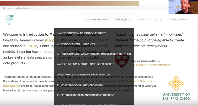
- Introduction to Machine Learning for Coders taught by Jeremy at fast.ai
- Machine Learning taught by Andrew Ng (on Coursera)
This is a good opportunity to introduce the course.
It’s a little outdated. But a lot of basic stuff still holds good.
It’s a foundation level course on Machine Learning. It doesn’t touch deep Learning at all. It is taught more of an academic way using a bottom-up approach.
Andrew Ng is a good teacher.
I would like to mention even we have an introductory Machine Learning course as well.
It’s twice as long as this one. It’s taught in top-down kind of code first approach.
It contains validation sets, interpretation and a lot of foundational courses.
It’s not a prerequisite but great to understand basic topics in ML.
Introduction to Machine Learning for Coders taught by Jeremy
Productionizing your models:
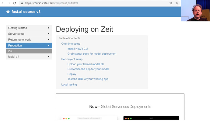
One thing you might now notice that there is production.
Right now there is just one platform Zeit
There is a guide as well.
Its frontend is Javascript
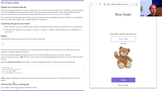
Jeremy was able to put his teddy bear detection model on Zeit.
Web Apps created by students:
- Edward Ross made “What car is that”?
Simply tested using a phone. - C Werner has created a guitar classifier
- You can decide whether your food is healthy or not.
- Trinidad and Tobago is home of Hummingbird, so you can click pictures of hummingbird and this model will name the bird species for you.
- Whether to eat a mushroom or not.
- 36 cousin classifier
- American Sign Language classifier by feeding signs from a webcam.
- Henry Palacci built yourcityfrom.space
- Alena Harley built a Tumor classifier. It’s a Computer vision approach that was initially not imaged.
What are we gonna do today?
We are going to build a lot of different applications
A. Multilabel prediction with Planet Amazon dataset on Kaggle.
lesson3-planet.ipynb
Kaggle competition page
It’s a satellite imaging dataset, Its fertile area in Deep Learning. Anything you can do with DL is just scratching the surface.
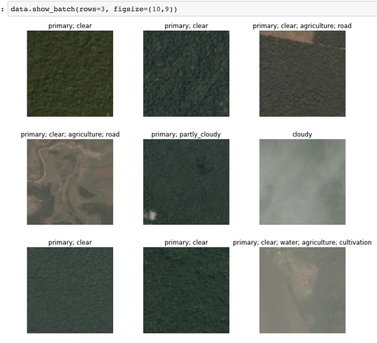
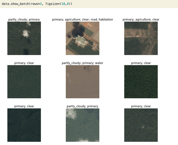
It looks like below:
They are small tiles from satellite images. Each one has got several different labels.
Label represents
- Weather: cloudy, partly cloudy
- primary - primary rainforest
- agriculture, roads
More details on Kaggle competition page
This is different than our previous classifier since this is not just one label. There can be more than one label to predict for a single image.
Kaggle is a competition website for Machine Learning and Deep Learning real-world problems. You can compete there and try to aim to rank on at least 10% on the leaderboard.
Downloading data
To install stuff from Kaggle you have to download the Kaggle API tool.
In Jupyter notebooks you will find commented lines, you can uncomment and run them
# ! pip install kaggle --upgrade
Then you need to upload your credentials from Kaggle on your instance. Login to Kaggle and click on your profile picture on the top left corner, then ‘My account’. Scroll down until you find a button named ‘Create New API Token’ and click on it. This will trigger the download of a file named ‘kaggle.json’.
Upload this file to the directory this notebook is running in, by clicking “Upload” on your main Jupyter page, then uncomment and execute the next two commands (or run them in a terminal).
#! mkdir -p ~/.kaggle/
#! mv kaggle.json ~/.kaggle/
You’re all set to download the data from planet competition. You first need to go to its main page and accept its rules. And run the two cells below (uncomment the shell commands to download and unzip the data). If you get a 403 forbidden error it means you haven’t accepted the competition rules yet (you have to go to the competition page, click on Rules tab, and then scroll to the bottom to find the accept button).
path = Config.data_path()/'planet'
path.mkdir(exist_ok=True)
path
How to label data images??
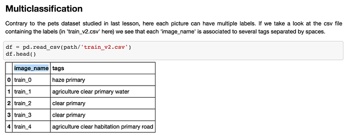
Kaggle provided a list of all labels in a CSV file.
We will use the Pandas library to read a CSV file.
This is how it reads.
We have to create databunch out of it. Once we have Databunch we can use show_ batch to view data and create CNN on it and learner on it to train the model.
Creating Databunch
This is the trickiest step to getting data in the format you can train your model later on.
So far we have shown you a few ways of doing it using factory methods in the last weeks. But there are so many choices we have to make where to save the file, which structure it should be and how does label appears, how do you transform it and so on.
We at fast.ai have got this Unique API called Data Block API, that Jeremy is very proud of.
There are many ways shown to bring in data in the correct format model can accept.
Let’s start by defining paths and splitting data into train and valid.
np.random.seed(42)
src = (ImageFileList.from_folder(path)
       .label_from_csv('train_v2.csv', sep=' ', folder='train-jpg', suffix='.jpg')
       .random_split_by_pct(0.2))
We have got an Image list in a folder, they have sep=’ ’ as space in between labels.
They are in a train-jpg folder and they have this suffix ‘.jpg’. We have randomly split out our data for validation by 20 percent.
tfms = get_transforms(flip_vert=True, max_lighting=0.1, max_zoom=1.05, max_warp=0.)

data = (src.datasets()
        .transform(tfms, size=128)
        .databunch().normalize(imagenet_stats))
Pay attention to the specific data augmentations applied here as seen in the parameters of get_transforms. flip_vert=True because for satellite image the specific orientation should not matter. max_lighting=0.1 and max_zoom=1.05 are what Jeremy finds to work the best with such images.
max_warp will change the perspective of the picture. It is handy when it comes to datasets like pets and cars, which clearly can be viewed from different perspectives; you can look at the dog from atop, or on the same level when staying close to the ground and playing with it. But for satellite, it always views the ground from the same perspective–high up above the ground in the space. Thus, adding a perspective warp to the training dataset will make it unrepresentative of real satellite images.
We are next going to create Dataset and transform them with transformation defined as tfms(in the 1st cell)
which is going to create DataBunch out of that which is then going to normalize data using ImageNet statistics.
PyTorch Concepts
I am going to now introduce you to the What are the Pytorch Objects or Classes that we are going to need.
You are gonna see them all the time in the Pytorch and fast.ai docs.
1. DataSet
Below is the source code of DataSet class
It Actually does nothing at all.
DataSet defines two things:
__getitem__()__len()__
In Python, this__<SOMETHING>__(Note there are two underscores at the start as well as in the end) are special methods with special behaviors.
You can look at these specific methods in Pytorch docs.
__getitem__() means object can be indexed with brackets.
o[3] gets you the fourth object in the dataset. where 3 is the index in the function definition. Note indexing starts from 0.
__len__() means if you call len(o) it will give you the length of total images in the dataset.
Both are raising NotImplementedError.
It means although You have to tell Pytorch about your data, you need to create a DataSet. It doesn’t do anything to help you to create a DataSet. It just defines what the dataset needs to do.
In other words, it just defines which is the 3rd item in my dataset(getitem()) and how much big is my dataset(len())?
Fast.ai has a lot of subclasses that do that for all different kinds of data stuff.
So far we have seen Image Classification Datasets. These are the datasets where getitem() will return an image and single label of that image.
So that’s what a dataset is. Now just dataset is not enough to train the model.
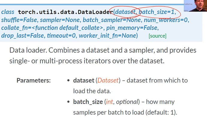
2. Data Loader
The first thing we have to do if you remember last week’s Gradient Descent Tutorial is we have to have few images or few items at a time so that GPU can work in parallel.
Remember we do this thing called minibatch. Minibatch is a few images we present to a model at a time that can be trained in Parallel.
So to create a minibatch we use another Pytorch class called a DataLoader
DataLoader takes Dataset in its Constructor. So; its gonna get the 3rd item, 6th item or the 20th item, it’s gonna grab items at random. And create a batch of whatever size you want and send it to GPU.
DataLoader is something that grabs individual items combines them into a mini-batch and sent over to GPU for training.
So you can see from the argument list there are already a lot of choices you have to make.
What kind of Dataset am I creating, where its data is going to come from? For Dataloader what should be the batch size.
3. DataBunch
This still isn’t enough to train a model. Because we have no way to validate. Before we had was a training set
We need a separate set of holdout data called a validation set. We will see how its gonna look.
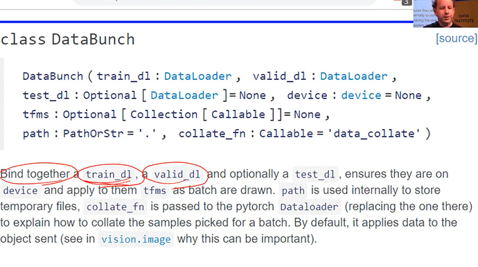
So for that, we use the fast.ai class called DataBunch.
A DataBunch is something that binds together a training data loader and a validation data loader.
When you look at fast.ai docs, if you don’t know what is the variable/symbol be used for you can look up elsewhere. In the class argument list, you can see train_dl is a dataloader. (argument : Type)
So when you create a DataBunch, you are giving a train and valid dataloaders. And that is now an object that you can send off to a learner. Then it will start learning. That was basic stuff.
Coming back to the code
src = (ImageFileList.from_folder(path)
       .label_from_csv('train_v2.csv', sep=' ', folder='train-jpg', suffix='.jpg')
       .random_split_by_pct(0.2))

data = (src.datasets()
        .transform(tfms, size=128)
        .databunch().normalize(imagenet_stats))
These 2 lines are creating DataSet
Dataset returns 2 things, index of an image and label.
ImageList.folder => where do the images come from List of Image files which are in some folder
label_from_csv => where do the labels come from
random_split_by_pct => by how much to split them into train and validation
src.dataset => converts them into Pytorch DataSets
transform(tfms, size=128) => transforms images
DataBunch => This is actaully going to create Dataloaders in one go.
Examples of Data Block API
Let’s look at some examples of Data Block API because once you understand Data Block API you are never being lost.
Quoting from Data Block API docs :
The data block API lets you customize how to create a
DataBunchby isolating the underlying parts of that process in separate blocks, mainly:
1. MNIST dataset
If you are looking at MNIST which remember the pictures and classes of handwritten numerals.
You can do something like this:
- ImageFileList → What kind of dataset is this gonna be? It’s gonna be some list of image files
- from_folder → which are in some folder
- label_from_folder → and they are labeled according to the folder name they are in. For example, 3 or 7
- split_by_folder → and then we are going to split it into train and validation according to the folder they are in train and validation.
- add_test_folder() → you can optionally add a test set, will be discussed later in the course
- datasets() → will then be transformed into Pytorch datasets.
- transform() → transform them using
tfms = get_transforms(do_flip=False)and resize them into size=224/ - databunch() → and we going to convert them into a databunch.
Each of these stages inside these parentheses you can pass parameters to customize how that all works.
But in the case of this MNIST Dataset, all the defaults pretty much works!
So here, you can check. Let’s grab something.
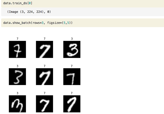
data.train_ds is the dataset. we can index into it so it calls particular here 1st record.
**data.train_ds[0]**
(Image (3, 224, 224), 0)
It gives an image of size 224 X 224 and with 3 color channels. Here is the result of it.
These are valid classes that are there 3 and 7. This is cut down a sample of MNIST.
data.valid_ds.classes
['3', '7']
2. Planet dataset
Here is an example using Planet dataset.
we are using a little subset of it, to make it easy to try things out.
planet = untar_data(URLs.PLANET_TINY)
planet_tfms = get_transforms(flip_vert=True, max_lighting=0.1, max_zoom=1.05, max_warp=0.)
data = ImageDataBunch.from_csv(planet, folder='train', size=128, suffix='.jpg', sep = ' ', ds_tfms=planet_tfms)
With the data block API we can rewrite this like that:
data = (ImageFileList.from_folder(planet)
        #Where to find the data? -> in planet and its subfolders
        .label_from_csv('labels.csv', sep=' ', folder='train', suffix='.jpg')
        #How to label? -> use the csv file labels.csv in path,
        #add .jpg to the names and take them in the folder train
        .random_split_by_pct()
        #How to split in train/valid? -> randomly with the default 20% in valid
        .datasets()
        #How to convert to datasets? -> use ImageMultiDataset
        .transform(planet_tfms, size=128)
        #Data augmentation? -> use tfms with a size of 128
        .databunch())
        #Finally? -> use the defaults for conversion to databunch
Again we are grabbing data as
- ImageFileList → image files,
- from_folder → which are in some folder
- labels_from_csv() → this time labels are in csv called labels.csv.
- random_split_by_pct → and then we are going to split it into train and validation by setting default 20 percent aside for validation
- datasets() → will then be transformed into Pytorch datasets.
- transform() → transform them using
planet_tfms = get_transforms(flip_vert=True, max_lighting=0.1, max_zoom=1.05, max_warp=0.)
resizing into smaller size=128
8. databunch() → and finally creating a databunch.
There it is.
3. CAMVID dataset
Here are some more examples of another dataset we are going to look into today.
Camvid dataset is a set of pictures and every pixel in the picture is color-coded.
Loading the data
The images are in an ‘images’ folder and their corresponding mask is in a ‘labels’ folder.
camvid = untar_data(URLs.CAMVID_TINY)
path_lbl = camvid/'labels'
path_img = camvid/'images'
We have a file that gives us the names of the classes (what each code inside the masks corresponds to a pedestrian, a tree, a road…)
codes = np.loadtxt(camvid/'codes.txt', dtype=str); codes
array(['Animal', 'Archway', 'Bicyclist', 'Bridge', 'Building', 'Car', 'CartLuggagePram', 'Child', 'Column_Pole',
       'Fence', 'LaneMkgsDriv', 'LaneMkgsNonDriv', 'Misc_Text', 'MotorcycleScooter', 'OtherMoving', 'ParkingBlock',
       'Pedestrian', 'Road', 'RoadShoulder', 'Sidewalk', 'SignSymbol', 'Sky', 'SUVPickupTruck', 'TrafficCone',
       'TrafficLight', 'Train', 'Tree', 'Truck_Bus', 'Tunnel', 'VegetationMisc', 'Void', 'Wall'], dtype='<U17')
And we define the following function that infers the mask filename from the image filename.
This fubction basically tells whereabouts of colour coding of each pixel in different places.
get_y_fn = lambda x: path_lbl/f'{x.stem}_P{x.suffix}'
Then we can easily define a DataBunch using the data block API. Here we need to use tfm_y=True in the transform call because we need the same transforms to be applied to the target mask as were applied to the image.
data = (ImageFileList.from_folder(path_img)                #Where are the input files? -> in path_img
        .label_from_func(get_y_fn)                         #How to label? -> use get_y_fn
        .random_split_by_pct()                             #How to split between train and valid? -> randomly
        .datasets(SegmentationDataset, classes=codes)      #How to create a dataset? -> use SegmentationDataset
        .transform(get_transforms(), size=96, tfm_y=True)  #Data aug -> Use standard tfms with tfm_y=True
        .databunch(bs=64))                                 #Lastly convert in a databunch with batch size of 64.
4. COCO dataset
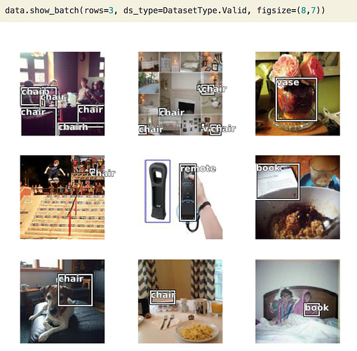
One more example, what if we want to create something like this. It has a vase, chair, remote control, book.
This is called as object detection dataset.
So we got a little minimum COCO dataset.
coco = untar_data(URLs.COCO_TINY)
images, lbl_bbox = get_annotations(coco/'train.json')
img2bbox = {img:bb for img, bb in zip(images, lbl_bbox)}
get_y_func = lambda o:img2bbox[o.name]
COCO is the most famous academic dataset for object detection.
data = (ImageFileList.from_folder(coco)
        #Where are the images? -> in coco
        .label_from_func(get_y_func)
        #How to find the labels? -> use get_y_func
        .random_split_by_pct()
        #How to split in train/valid? -> randomly with the default 20% in valid
        .datasets(ObjectDetectDataset)
        #How to create datasets? -> with ObjectDetectDataset
        #Data augmentation? -> Standard transforms with tfm_y=True
        .databunch(bs=16, collate_fn=bb_pad_collate))
        #Finally we convert to a DataBunch and we use bb_pad_collate
We will be again using a function here to grab labels of a dataset. We will convert it to ObjectDetectionDataset and we will create a databunch with batch size 16.
When we do object detection we have to generally use smaller batch size to avoid OOM error.
And we will learn we have to use something called collation function
collate_fn=bb_pad_collate
and once that is done we can call show_batch.
All these documentation is done through Jupyter notebooks. You can find them in fastai/docs_src folder. You can play along with parameters to better understand data block API.
And also it is there in the documentation on the fast.ai website docs.fast.ai.
You can use the search functionality to search for anything in docs.
Anything you want to use in fastai there is a documentation page as well jupyter notebook.
Back to Planet notebook
np.random.seed(42)
src = (ImageItemList.from_csv(path, 'train_v2.csv', folder='train-jpg', suffix='.jpg')
       .random_split_by_pct(0.2)
       .label_from_df(sep=' '))

data = (src.transform(tfms, size=128)
        .databunch().normalize(imagenet_stats))
we can do these 2 steps together, but you will learn in a moment why are we splitting it up.
Transformations
Flipping
tfms = get_transforms(flip_vert=True, max_lighting=0.1, max_zoom=1.05, max_warp=0.)
Let’s see function signature
Signature: get_transforms(do_flip:bool=True, flip_vert:bool=False, max_rotate:float=10.0,
max_zoom:float=1.1, max_lighting:float=0.2, max_warp:float=0.2, p_affine:float=0.75,
p_lighting:float=0.75, xtra_tfms:float=None) -> Collection[fastai.vision.image.Transform]
Transforms by default do flip randomly for each image, but they actually only flip them horizontally (left/right as in mirror image).
which makes sense, if you want to tell if it is a dog or a cat it doesn’t matter if its pointing left or right. But you wouldn’t expect it to be upside down.
On the other hand, for a case of satellite imagery, whether it is cloudy or primary or hazy, whether there is a road or not would be flipped upside down. So, for our case flip_vert which defaults to false, we are going to make it TRUE.
To say that ya randomly you should flip upside down.
It also doesn’t need to be just vertically. You can try all possible angles of 90 degrees rotations.
So there are 8 possible symmetries that it tries out. These are called dihedral symmetries.
Jeremy found these parameters work pretty well for Planet.
Warping
One that’s interesting is max_warp
Perspective warping is something fewer libraries provide and those that provide tends to be very slow.
Jeremy thinks fast.ai is the first one to provide a fast perspective warping.
This is interesting because if I look at you from below verses from above the kind of your shape changes.
So if you are taking a photo of a cat or a dog sometimes you will be higher you will be lower, then that kind of change of shape is certainly something you would want to include as you’re training your batch of images. You want to modify it a little bit each time.
Not for satellite images. A satellite always points straight down at the planet.
If you added perspective warping, you would be making changes that aren’t going to be there in real life. So he turns it off.
This is all called as Data augmentation.
We will see later during the course. But you can kinda get feel all that you could do to augment your data.
In general, the most important one is flip_vert. If you are looking at astronomical data or kind of pathology or digital slide data or satellite data where flipping vertical is possible you should set it to TRUE which will make your model generalize well.
So these were the steps necessary to create databunch.
Now to create satellite imagery multi-label classifier for each tile, it’s gonna figure out what is the weather, what is there in its road, water bodies.
There is nothing else to learn other than creating databunch.
The rest part of the learning is nearly the same as previous problems.
Define architecture and start training
First Jeremy tried resnet34, but later he found resnet50 worked little better.
We will use resnet50 architecture in this.
arch = models.resnet50

acc_02 = partial(accuracy_thresh, thresh=0.2)
f_score = partial(fbeta, thresh=0.2)
learn = create_cnn(data, arch, metrics=[acc_02, f_score])
One more change is there in the metric. Metric has nothing to do with how the model trains
- Acurracy
- f_score
We use metric for seeing how the model is performing on validation set. You can see below accuracy_threshold and fbeta metric values.
So if you want to figure out how to do your model perform better, changing metrics will never be something that you need to do there. They just show you how well are you going.
You can have 0 or more metrics to be printed out when your model is training.
For now, we want to know 2 things Accuracy and f_score, which is something Kaggle has asked for.
f_score
Kaggle uses this metric to score your predictions on planet data.
When you have a classifier you going to have some false positives and false negatives. How do you weigh up those two things? You have to kinda create a single number from those two.
Lots of different ways to do that.
f_score is a nice way fo combining that into a single number.
There are various types of f_score functions like f1 score, f2 score, etc.
We have
fbeta()

Signature: fbeta(y_pred:torch.Tensor, y_true:torch.Tensor, thresh:float=0.2, beta:float=2, eps:float=1e-09, sigmoid:bool=True) -> <function NewType.<locals>.new_type at 0x117615950>
Docstring: Computes the f_beta between preds and targets
File:      ~/anaconda/envs/fastai/lib/python3.6/site-packages/fastai/metrics.py
Type:      function
So as you can see in the signature of fbeta() function beta value defaults to 2
i.e f2 score. Kaggle says this in the evaluation metric. So no need to change that.
We need to set threshold, what is it?
If you look at the source code of accuracy.
??accuracy

Signature: accuracy(input:torch.Tensor, targs:torch.Tensor) ->
<function NewType.<locals>.new_type at 0x117615950>
Source:
def accuracy(input:Tensor, targs:Tensor)->Rank0Tensor:
    "Compute accuracy with `targs` when `input` is bs * n_classes."
    n = targs.shape[0]
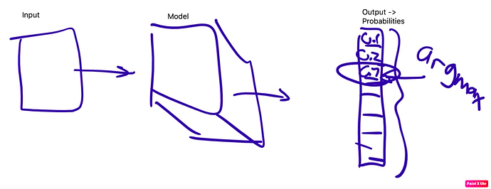
    input = input.argmax(dim=1).view(n,-1)
    targs = targs.view(n,-1)
    return (input==targs).float().mean()
File:      ~/anaconda/envs/fastai/lib/python3.6/site-packages/fastai/metrics.py
Type:      function
input is input.argmax
In the output, we have 10 probabilities for 10 classes of MNIST.
We have to find out which is the biggest and return its index. In python, that is done by argmax() function.
then we have to compare that to actual here,
targs = targs.view(n,-1)
and then take the average.
return (input==targs).float().mean()
That was the accuracy.
We can’t use this metric for planet data since there are multiple labels to predict.
So, instead
Databunch has a special attribute called c
data.c
17
c is how many output probabilities we want to create.
So for any classifier, we want 1 probability for each class.
In other words, data.c is always gonna equal to len(data.classes)
Threshold
38:20
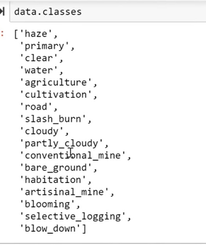
So we are not going to pick 1 of those 17, instead, we are gonna pick n of 17.
We compare each probability to some threshold.
If something has a higher probability than the threshold, we can assume it has that feature. and we can pick that threshold. Jeremy found that for this dataset a threshold of 0.2 works well. You can experiment to find a good threshold.
So Jeremy decided to print out accuracy with the threshold of 0.2
Normal accuracy function cannot do that. It can’t argmax. We have to use a different function called accuracy_thresh(). So this one will compare all probabilities with a threshold and return the ones which are higher than the threshold.
??accuracy_thresh()

Signature: accuracy_thresh(y_pred:torch.Tensor, y_true:torch.Tensor, thresh:float=0.5, sigmoid:bool=True) -> <function NewType.<locals>.new_type at 0x117615950>
Source:
def accuracy_thresh(y_pred:Tensor, y_true:Tensor, thresh:float=0.5, sigmoid:bool=True)->Rank0Tensor:
    "Compute accuracy when `y_pred` and `y_true` are the same size."
    if sigmoid: y_pred = y_pred.sigmoid()
    return ((y_pred>thresh)==y_true.byte()).float().mean()
So our metric will be calling the funtion for us so we can’t set any threshold.
We will use a special function to call accuracy_thresh with threshold=0.2.
We can do that below way
Partial function application in python 3
It’s common to define a new function that just like an old function but always gonna be called with a particular parameter. In python, this is called the partial function.
acc_02 = partial(accuracy_thresh, thresh=0.2)
The partial function takes some function and keyword and values and creates new function acc_02 i.e exactly same as accuracy_thresh, but it is always gonna get called up with thresh=0.2.
Choosing learning rates
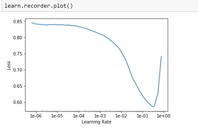
Then we can go ahead and do the regular stuff lr.find(), learn.recorder.plot()
Find the thing with the steepest slope.
we can choose the learning rate somewhere around 1e-2.
And then fit for a while and check accuracy.
We got 96 % accuracy and fbeta value of 0.926.
If you go to kaggle leaderboard and see score first 50 ranks have a score of 0.93. So we can say that we are on the right track. There is very little extra to do most of the time.
Question 1:
When your model makes an incorrect prediction in a deployed app, is there a good way to record that error and use that learning to improve the model in a more targeted way?
Answer:
Ya. There is a way to record that. Thays up to you. Maybe some of you can try this week.
You need to have your user tell you that you were wrong. This Australian car your model predicted was Holden but it is a Falcon. You have to take that feedback.
You need to record in logs somewhere. This was a file, stored here, the prediction made, this is actual feedback I got. Then at the end of the day, you can set up a little job to run something or manually do the job. And do fine-tuning.
what does fine-tuning look like??
Let’s pretend we have saved this model and then we unfreeze and then we fit a little bit more.
learn.save('stage-1-rn50')
learn.unfreeze()

learn.lr_find()
learn.recorder.plot()

learn.fit_one_cycle(5, slice(1e-5, lr/5))
Here in the planet notebook, Jeremy is fitting the model to the original dataset.
But we can create a new DataBunch, with just the misclassified images. and go ahead and fit.
And misclassified ones will be likely to be more interesting, so you want to use a slightly higher learning rate to make the kind of minimal or you want to run a few more epochs.
You just call fit with your misclassified images and passing incorrect ones
This should help your model.
Question 2: 44:01
Can you talk more about Data Block Ideology? Not quite sure how the blocks are meant to be used. Do they have to be in a certain order? is there any other library that uses this type of programming that I can look at?
Answer: Yes, they do have to be in a certain order. This is you see the order in examples of use.
- What kind of data do you have
- Where does it come from?
- how do you label it
- how do you split it
- what kind of datasets do you want
- optionally how do I transform it
- and then how do I create a DataBunch from it.
So these are the steps.
This kind of approach you tend to see more in ETL software, where this kinda particular stages in pipeline occur.
What you need to do is use this example to guide you and then look up the documentation to see which particular kind of application you want and what are the Data Block API pieces available for that kind of application.
You can look at source code if you got a completely new application to create your part of any of those steps.
You can play around to get a good sense of it.
Question 3:
47:39
What resources do you recommend to getting started with video, for example, being able to pull frames and submit them to your model?
Answer:
It depends. If you are using the web, then there are web APIs, you can grab frames using web APIs and there are just images you can pass along.
Most people using OpenCV. We can add in lesson wiki if people know any more resources.
Back to choosing learning rates
As usual, we unfreeze and fit some more and we got fbeta 0.929 ish
One thing to notice here is before we unfreeze, plot learning rate finder output. you tend to get this shape Find the steepest slope, not at the bottom, because you will slide down off quickly. If you choose bottom value it’s gonna send you much up.
So you choose lr somewhere in the middle of the steepest slope.
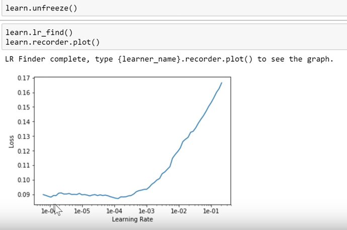
And then again after unfreeze, you generally get a very different shape.
So Jeremy generally looks up for a point where immediately it shoots up, and from there go back like 10 steps and choose that so 1e-5. It’s a kind of rule of thumb.
learn.fit_one_cycle(5, slice(1e-5, lr/5))
That’s for the 1st half of layers slice and for the second half Jeremy chooses the previous lr used for the frozen part and divides it by 5 or 10. So lr which was lr=0.01 that gets divided by 5 i.e, lr/5
How to get a score better than 0.929 ? → Transfer learning
Here is the trick.
data = (src.transform(tfms, size=128)
        .databunch().normalize(imagenet_stats))
- When Jeremy created the dataset, he put size=128, and actually images kaggle gave us are 256.
So Jeremy used size 128 partially coz he wanted to experiment quickly. It’s much easier to use smaller images to experiment but the second reason is he now has a model that’s pretty good at recognizing the context of 128 X 128 satellite image tiles.
So now he creates using 256 X 256 images. So why not to use transfer learning?
So he starts with a model i.e good at 128 X 128 images and fine-tune that only. Don’t start again from scratch.
So that’s gonna be interesting if I have trained my model a lot and I’m on the verge of overfitting than I don’t want to do it. But then I will be creating a whole new Dataset, One way my images are twice the size on each axis, so 4 times bigger.
So it’s a different dataset as far as Convolutional Neural Network is concerned. So we can’t lose all that overfitting. We get to start over again.
So Let’s create a new DataBunch for the same learner, where the DataBunch is 256 X 256 instead.
Creating new DataBunch with image size =256
Let’s look at the code for doing this.
data = (src.transform(tfms, size=256)
        .databunch().normalize(imagenet_stats))
Take that source src which is same as below:
src = (ImageItemList.from_csv(path, 'train_v2.csv', folder='train-jpg', suffix='.jpg')
       .random_split_by_pct(0.2)
       .label_from_df(sep=' '))
and transform it with same tfms
tfms = get_transforms(flip_vert=True, max_lighting=0.1, max_zoom=1.05, max_warp=0.)
But this time use size=256.
Now that should be better anyway because
- These are higher resolution(256 X 256 instead of 128 X 128) images
- We haven’t got rid of our learner, we will be using the same old learner we had before. So we are gonna start with this pre-trained model.
We just have to replace the data inside the same learner with this new DataBunch.
learn.data = data
data.train_ds[0][0].shape
Out[ ]:  torch.Size([3, 256, 256])
And then we will freeze it again,
learn.freeze()
That means we are going back to just training the last few layers. and we will do a new lr.find()
And because now we have a pretty good model. Good for 128X128. So probably it gonna be at least Ok for 256X256 sizes.
We can’t see that same sharp steepest slope here as we have seen before. But we can certainly see where its gonna get shot up. So Jeremy is gonna pick something which is way before its gonna go too high i.e 1e-2
lr=1e-2/2
learn.fit_one_cycle(5, slice(lr))
So we will be training some more time, fiddle with it a bit more. And as we can see very quickly we are up to 0.92 at our previous score and we pass 0.93. And now if you see on Kaggle leaderboard. we are in the top 10%.
We have hit our first goal. We are doing the very least pretty competent at the problem of breaking this satellite imagery problem.
Now again we can unfreeze and train a little more. we get a score of 0.9314. That will take you in the top 25 in Kaggle leaderboard. For this, you have to download a test set from Kaggle, predict that and submit it to Kaggle using Late submission And see where you stand.
Saving the model weights
As you can see Jeremy tries to save things as he tends to go longer.
learn.save('stage-2-256-rn50')
And name it appropriately to know whether it was before or after unfreeze, what was the image size, what was the architecture used.
So that was Planet, Multi-label classification problem.
CamVid Image Segmentation
Another example we are gonna look at is this dataset called CamVid, and here we will be doing Segmentation.
What is segmentation?
We will start with the picture like this,
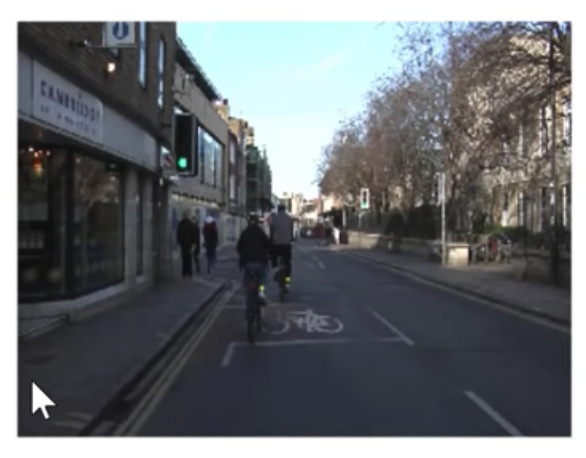
and we gonna create a color-coded picture like this.
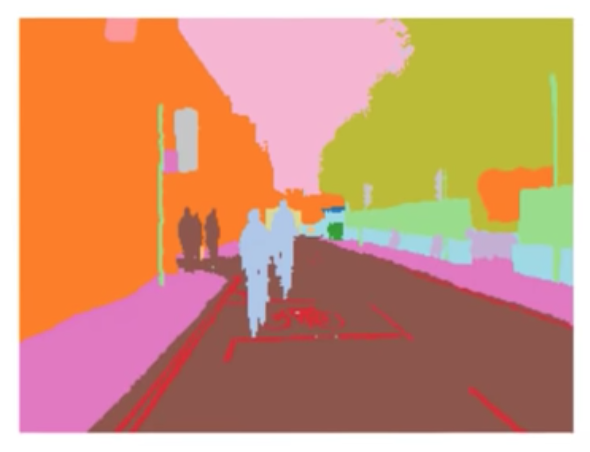
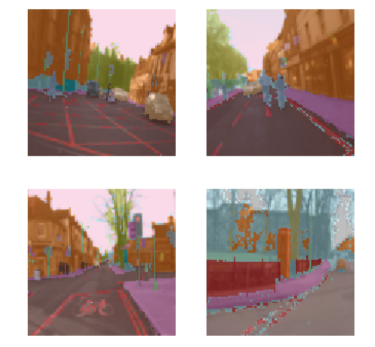
Where all of the bicycle pictures are in the same color, all of the road line pixels are in the same color, all of the tree pixels or building pixels are in the same color. The sky is in the same color. and so forth.
We are not going to make them color but we are going to do it
Where each of those pixels has a unique number.
So, in this case, the top left is building so the building has got number 4, top right is a tree so the tree is 26. etc
In other words, this single top-left pixel, Jeremy mentions this. We are gonna do a classification problem like the pets classification for the very top left pixel. We are gonna say what is that top left pixel? Is it a bicycle, road lines, sidewalk, or building. What is the very top left pixel? And then what is next pixel along.
So we are gonna do a little classification problem for every single pixel, in every single image. So that is called Segmentation.
To build a Segmentation model, you need to download or create a Dataset, where someone has labeled every pixel. So as you can imagine that’s a lot of work.
You probably not gonna create your segmentation dataset. You gonna find them or download from somewhere.
This is very common in medicine or life sciences. If you looking into slides or nuclei, you already have a whole bunch of segmented cells or nuclei. If you are in Radiology, you probably have lots of examples of segmented legions and so forth.
So there are a lot of different domain areas where there are domain-specific tools for creating these segmented images. From this example, you can guess in self-driving cars and stuff like that where you need to see what kins of objects are around and where are they.
In this case, there is a nice dataset called CamVid, which we can download they have already images and segment masks prepared for us.
Fast.ai maintained Datasets
![]() Remember, pretty much all of the datasets we have provided inbuilt URLs for, like here URLs.CAMVID you can see their details at fast.ai datasets page.
Remember, pretty much all of the datasets we have provided inbuilt URLs for, like here URLs.CAMVID you can see their details at fast.ai datasets page.
Nearly all of them are academic datasets, where some very kind people have created for us. So we can use these datasets. If you do use these datasets for one of your projects. You should give them credits using the citation. Because they have gone through all the trouble of creating it. If you click the link in the citation, it will direct to the original academic paper.
Question:
01:00:27
Is there a way to return a suitable learning rate number directly by lr.find(), instead of plotting and visually inspecting that vale? How to read lr finder plot better()
Answer: The short answer is NO. We don’t have lr finder returning a number directly not now.
How you read an LR finder graph depends on what stage you are at, what shape of it is. When you are just training head, before you unfreeze, it always looks like this.
And you could certainly create something smooth version of this.
Look for the steepest negative slope and picked that, you will be fine nearly all the time.
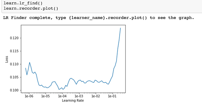
But these kinds of ones,
you need to do some amount of experimentation.
If the line is going up you don’t want it, almost exactly at the bottom also you have to discard, because you need it to be going downwards. But if you start somewhere around 10x smaller than that, something smaller than that, try a few numbers to find out which one works best.
Within a few weeks, you will find yourself picking the best learning rate.
Maybe someone can pick this as a project to generate an auto-learning rate finder. Collect all datasets, try to come up with heuristics, compare with lesson notebooks and come up with reliable lr.
We haven’t got there yet.
Back to segmentation
So, How do we do Image Segmentation? Like everything else.
We start with getting data in
path = untar_data(URLs.CAMVID)
path.ls()
Out[ ]:
[PosixPath('/home/ubuntu/course-v3/nbs/dl1/data/camvid/images'),
 PosixPath('/home/ubuntu/course-v3/nbs/dl1/data/camvid/codes.txt'),
 PosixPath('/home/ubuntu/course-v3/nbs/dl1/data/camvid/valid.txt'),
 PosixPath('/home/ubuntu/course-v3/nbs/dl1/data/camvid/labels')]
There is a folder called labels and images. So we will crate paths for each of those.
path_lbl = path/'labels'
path_img = path/'images'
Take a look inside
fnames = get_image_files(path_img) fnames[:3]

Out[ ]:

[PosixPath('/home/ubuntu/course-v3/nbs/dl1/data/camvid/images/0016E5_08370.png'),
PosixPath('/home/ubuntu/course-v3/nbs/dl1/data/camvid/images/Seq05VD_f04110.png'),
PosixPath('/home/ubuntu/course-v3/nbs/dl1/data/camvid/images/0001TP_010170.png')]

In [ ]:

lbl_names = get_image_files(path_lbl) lbl_names[:3]

Out[ ]:

[PosixPath('/home/ubuntu/course-v3/nbs/dl1/data/camvid/labels/0016E5_01890_P.png'),
PosixPath('/home/ubuntu/course-v3/nbs/dl1/data/camvid/labels/Seq05VD_f00330_P.png'),
PosixPath('/home/ubuntu/course-v3/nbs/dl1/data/camvid/labels/Seq05VD_f01140_P.png')]
You can see here some kind of coded file names for images and for the segmented masks.
You have to figure out how to link two to each other.
You can look at Datasets README or their website to understand more about data.
Labels
If you look closely these images and labels file names have similarity except _P suffix for segmented masks.
So Jeremy created a little function to verify.
get_y_fn = lambda x: path_lbl/f'{x.stem}_P{x.suffix}'
And it worked. It was same structure.
Masks
Usually we open an image using open_image() and use .show() to display the images.
But as we described, this is not a usual image file that contains integers. So we have to use open_masks rather than open_image because we want to return integers, not floats. Fastai knows how to deal with masks, so if you go mask.show(), it will automatically color code it for you in some appropriate way. That’s why we said open_masks.
src_size = np.array(mask.shape[1:])
src_size,mask.data
Out[ ]:
(array([720, 960]), tensor([[[ 4,  4,  4,  ..., 26, 26, 26],
          [ 4,  4,  4,  ..., 26, 26, 26],
          [ 4,  4,  4,  ..., 26, 26, 26],
          ...,
          [19, 19, 19,  ..., 17, 17, 17],
          [19, 19, 19,  ..., 17, 17, 17],
          [19, 19, 19,  ..., 17, 17, 17]]]))
We can kind of have a look inside look at the data see what the size is so there’s 720 by 960. We can take a look at the data inside, and so forth. The other thing you might have noticed is that they gave us a file called codes.txt and a file called valid.txt.
codes = np.loadtxt(path/'codes.txt', dtype=str); codes
Out[ ]:
array(['Animal', 'Archway', 'Bicyclist', 'Bridge', 'Building', 'Car', 'CartLuggagePram', 'Child', 'Column_Pole',
       'Fence', 'LaneMkgsDriv', 'LaneMkgsNonDriv', 'Misc_Text', 'MotorcycleScooter', 'OtherMoving', 'ParkingBlock',
       'Pedestrian', 'Road', 'RoadShoulder', 'Sidewalk', 'SignSymbol', 'Sky', 'SUVPickupTruck', 'TrafficCone',
       'TrafficLight', 'Train', 'Tree', 'Truck_Bus', 'Tunnel', 'VegetationMisc', 'Void', 'Wall'], dtype='<U17')
code.txt contains a list telling us that, for example, number 4 is building. Just like we had grizzlies, black bears, and teddies, here we’ve got the coding for what each one of these pixels means.
How to create a databunch [1:05:53]
To create a data bunch, we can go through the data block API and say. - We’ve got a list of image files that are in a folder. We then need to split into training and validation. In this case, Jeremy doesn’t do it randomly because the pictures they’ve given us are frames from videos. If I did them randomly I would be having two frames next to each other: one in the validation set, one in the training set. That would be far too easy and cheating. So the people that created this dataset gave us a list of file names (valid.txt) that are meant to be in your validation set and they are non-contiguous parts of the video. So here’s how you can split your validation and training using a filename file. We need to create labels that we can use that get_y_fn (get Y file name function) we just created.
Datasets

size = src_size//2
bs=8

src = (SegmentationItemList.from_folder(path_img)
       .split_by_fname_file('../valid.txt')
       .label_from_func(get_y_fn, classes=codes))
From that, we can create our datasets.
We have a list of class names. Often with stuff like the planet dataset or the pets dataset, we have a string saying this is a pug, this is a ragdoll, or this is a Birman, or this is cloudy or whatever. In this case, you don’t have every single pixel labeled with an entire string (that would be incredibly inefficient). They’re each labeled with just a number and then there’s a separate file telling you what those numbers mean. So here’s where we get to tell the data block API this is the list of what the numbers mean. So these are the kind of parameters that the data block API gives you.
data = (src.transform(get_transforms(), size=size, tfm_y=True)
        .databunch(bs=bs)
        .normalize(imagenet_stats))
Here are our transformations. Here’s an interesting point. Remember Jeremy told you that, for example, sometimes we randomly flip an image? What if we randomly flip the independent variable image but we don’t also randomly flip the target mask? Now I’m not matching anymore. So we need to tell fastai that I want to transform the Y (X is our independent variable, Y is our dependent) I want to transform the Y as well. So whatever you do to the X, Jeremy also wants you to do to the Y (tfm_y=True). There are all these little parameters that we can play with.
We can create our data bunch. Jeremy is using a smaller batch size (bs=8) because, as you can imagine, He’s creating a classifier for every pixel, that’s going to take a lot more GPU right. He found a batch size of 8 is all he could handle. Then normalize in the usual way.
data.show_batch(2, figsize=(10,7))
