📝 Deep Learning Lesson 2 Notes

PoonamV · October 31, 2018, 9:03am

This is a forum wiki thread, so you all can edit this post to add/change/organize info to help make it better! To edit, click on the little pencil icon at the bottom of this post. Here’s a pic of what to look for:

<<< Notes: Lesson 1 ｜ Notes: Lesson 3 >>>

Practical Deep Learning for Coders v3 Lesson 2

Hi, welcome to the 2nd lesson.
We are going to take a deeper dive into computer vision applications.

Official resources:

Jeremy made a few changes to the forums so that things will be smooth for everybody.

YouTube chat for remote students won’t be monitored, but you are encouraged to chat amongst yourself.
Anybody wants to ask important question/doubt, you should ask on forum topic lesson chat thread.
There is an advanced category, to ask an advanced question for the students who already have done Deep Learning. For example, discussion about arXiv paper, low level queries about the fastai library.
The things that we have not covered yet in the v3 course should go into the advanced category.
The in-class discussion thread is for discussing doubts during the lecture.
This thread will be read later also. If you want to ask the same question, you can upvote() it.
The question with more than 8 upvotes will be discussed during the lecture.

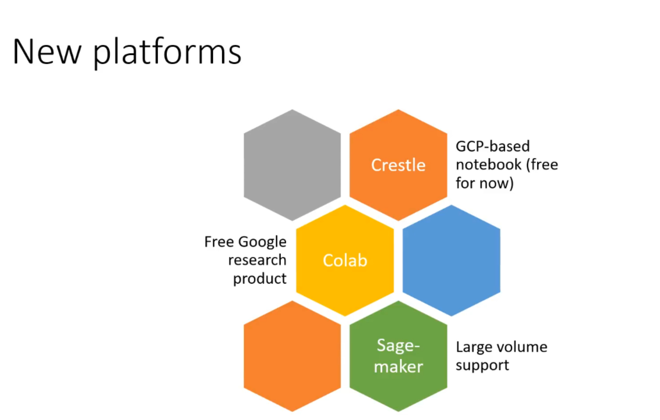
New Platforms

Crestle.ai is a lot like Gradient. It’s completely free for the next few weeks. So utilize it to the fullest.
Crestle creators will be there to answer your questions.
Colab is a free tool from Google.
You don’t need to spend a single dollar, but it’s not as smooth as other options.
Some of the students have created guides to set up your instance.
Sagemaker
Supports really large volumes. You can specify how big the system you need while creating an instance.
You can use aws credits you have got if you are in the in-person course.

Reminder: Always follow these 2 posts on the forums

The FAQ is a closed thread means only admins can edit it and post updates to it.
You should keep a close eye on it since fastai library and course notebooks are in actively developing stage. Most of the changes in them will be notified here in this thread.

In the platforms section, there are setup guides and discussion thread for each platform. Jeremy suggests to follow those guides and ask the question on particular discussion threads and not to open a new thread for platform related questions. So, that we can have everything in one place and your question will get answered quickly by platform experts.

Lesson 1 official resources and updates

It’s a wiki thread, that means every one of us can edit and update it.
You can watch it, it will have all the resources like video, notebook and so forth for the particular lesson.

How to watch a thread (Get notified)?

One way is to go to a particular thread like official updates one and click at the bottom on watching.
Another way to get mails is to click on your username in the top right corner and tickmark on send emails in Email section.

Summarizing the topic

Even after 1 week, the most popular thread has got over 1.1 k replies. That’s intimidatingly large.

We shouldn’t need to read every single one of them, you can choose to summarize that topic for you.

It will show you the ones with most likes ( ) and rest will be hidden in between.
Our role is to like important replies, so it will be more visible to others.

Always start your work by updating repo for course-v3 and fastai library

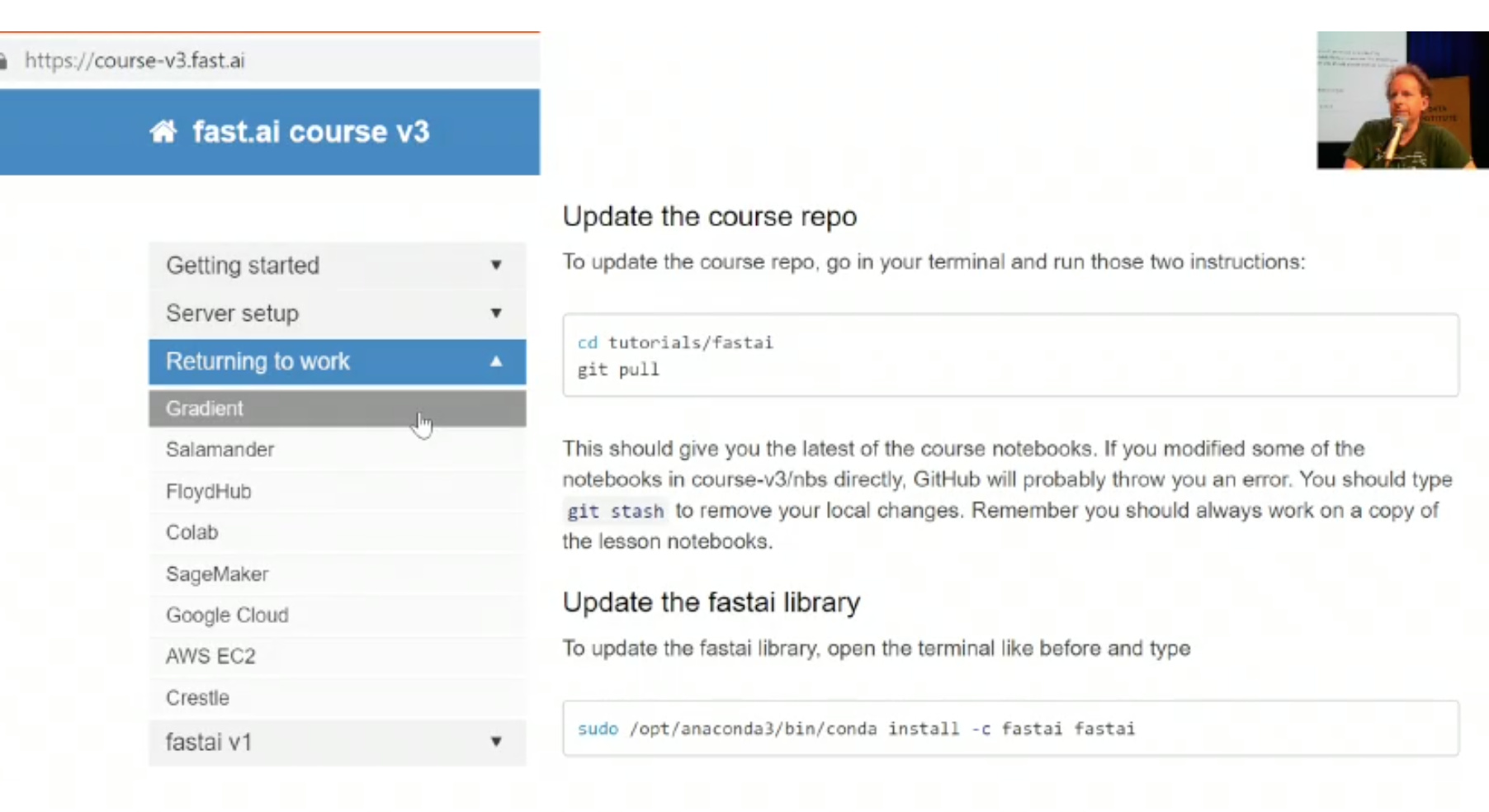
When you return the work

go to course documentation
choose the platform you are using
follow the 2 instructions to make sure you got latest Python notebooks and latest library.

Since fastai library and course notebooks are in actively developing stage. This is a very important step if you want to stay up-to-date.

This can slightly differ from platform to platform so make sure you execute instructions for your particular platform.

This will make everything smooth for you. But still if things not working for you, just delete the instance and start again if there is not mission critical stuff uploaded there. Don’t be afraid to ask on forums, if it’s not being asked already.

What other students have been doing this week

Share your work here thread.

167 people have shared their creations there.
How cool is that!. It’s pretty intimidating to put yourself out there, even you are new to this.

Figuring out Who’s talking in audio files?. Is it Ben Affleck or Joe Rogan.
Cleaning up WhatsApp files.
Ethan Sutin got new SoTA 80.5% accuracy over old benchmark of 79%.

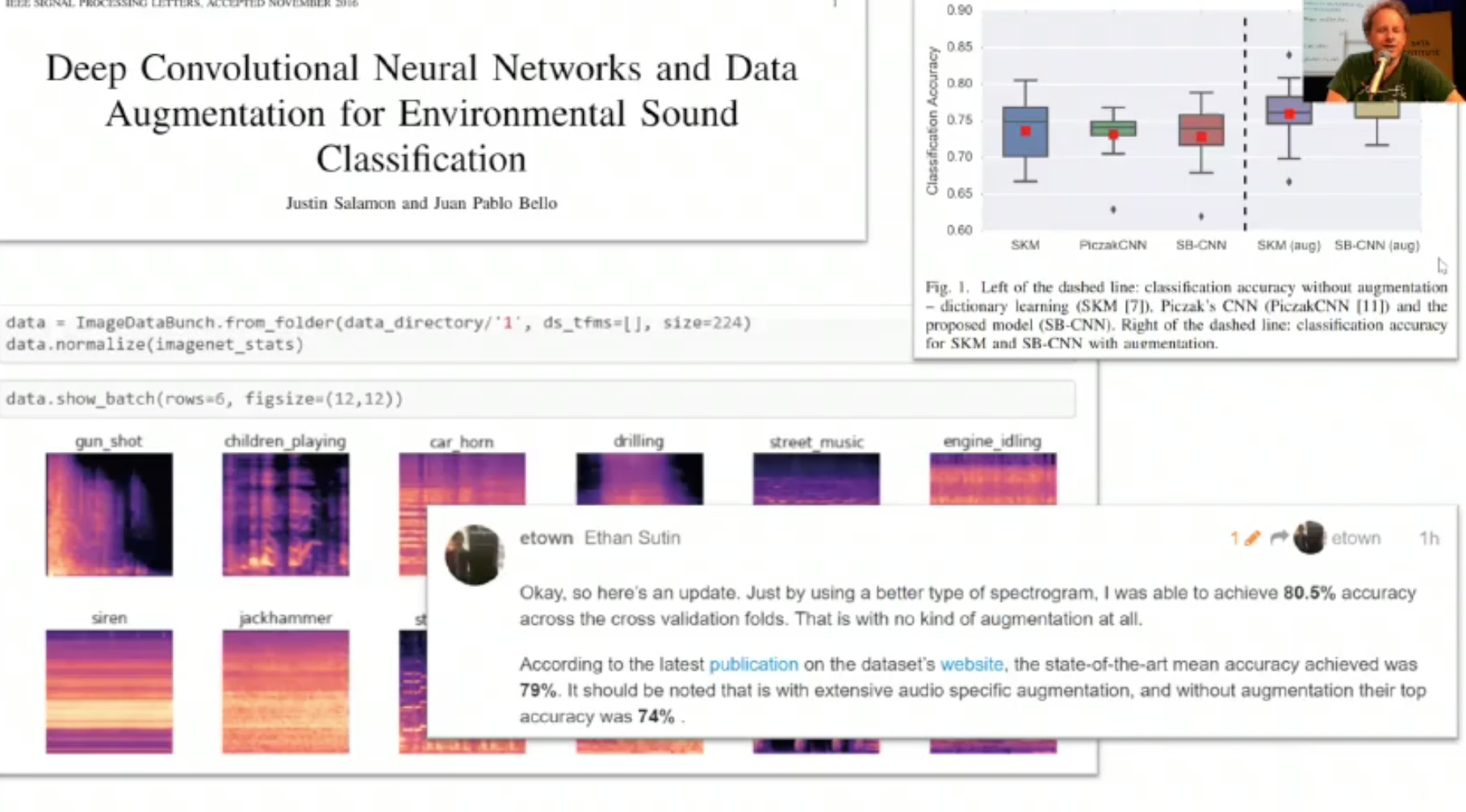
Turning sounds into pictures is a cool approach.

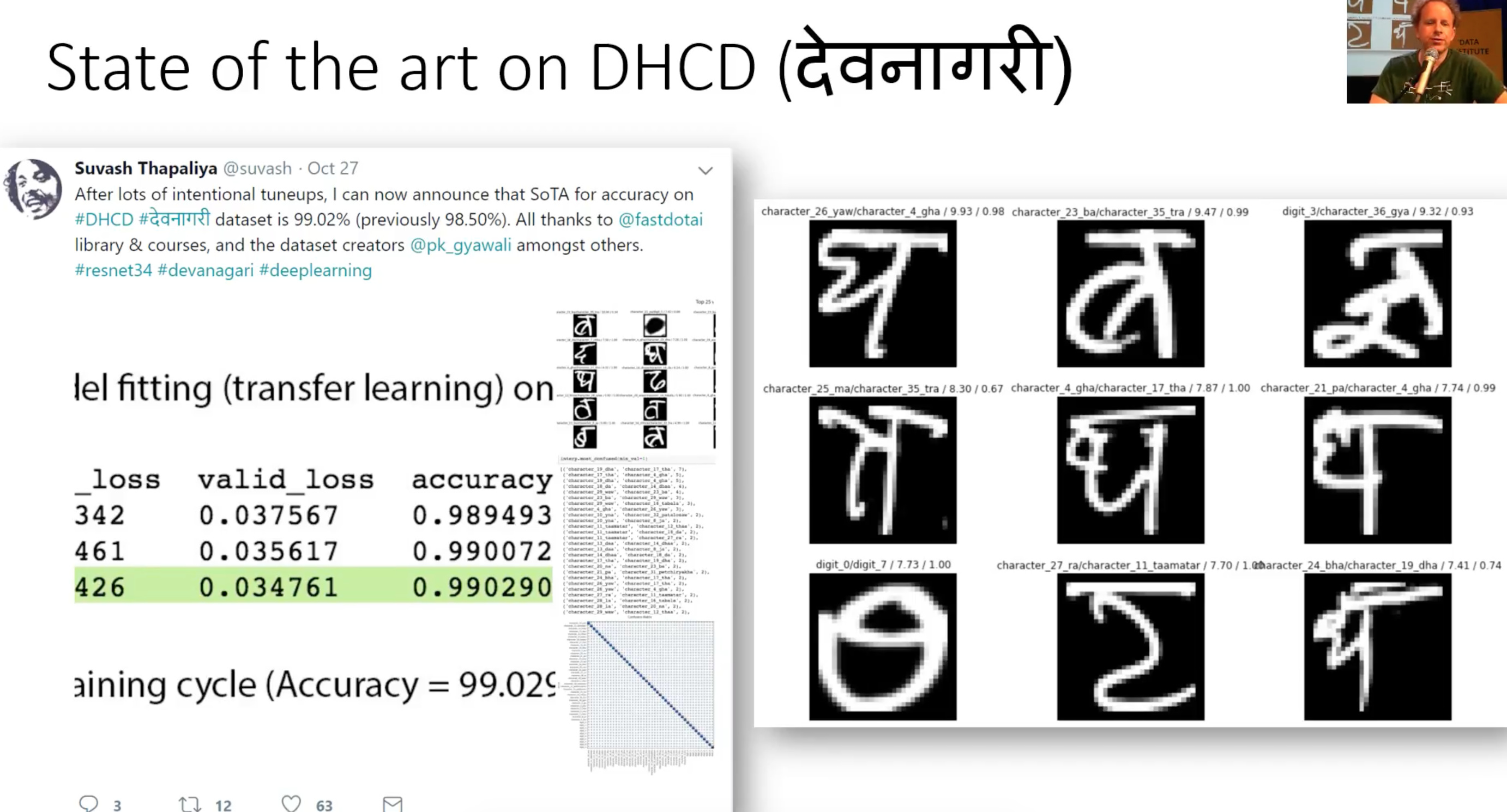
Suvash got new SOTA of 99.02% accuracy on Devanagari script dataset

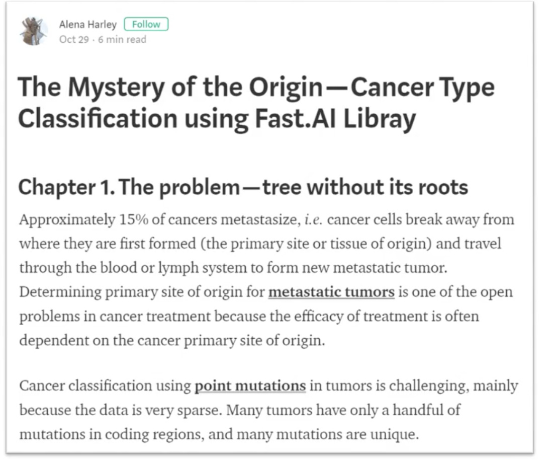
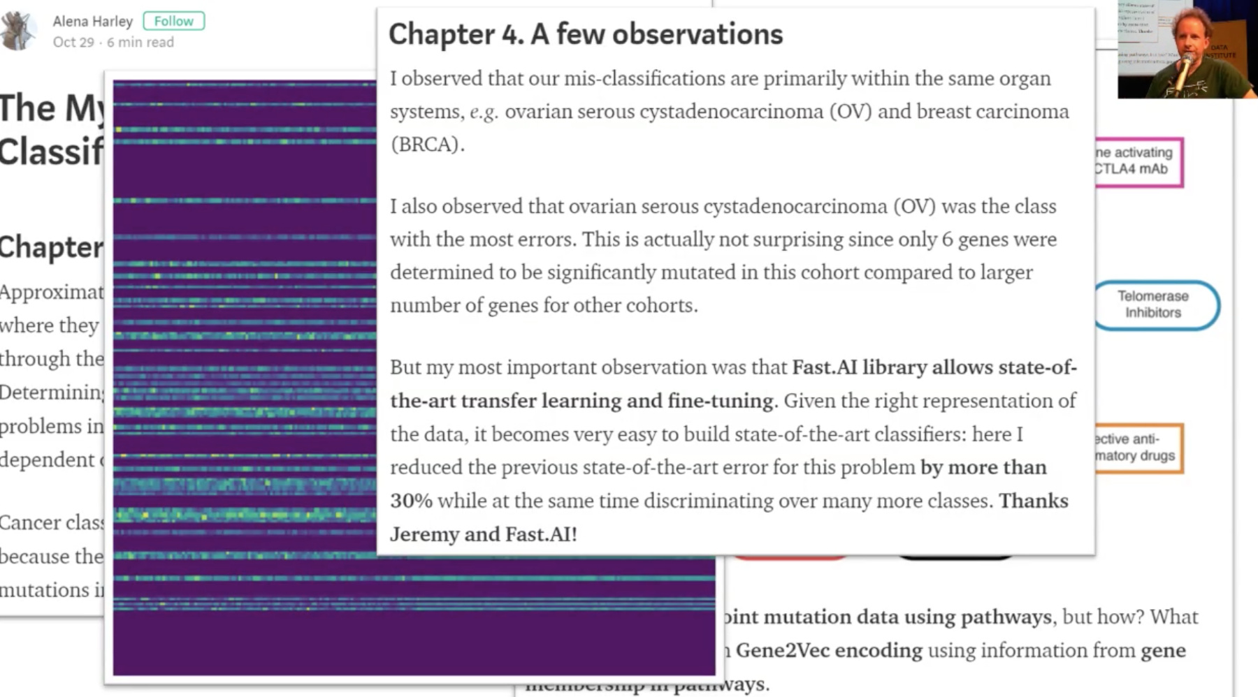
Alena did cancer classification using point mutations, which she turned into pictures.
She got more than 30% results over the previous benchmark.

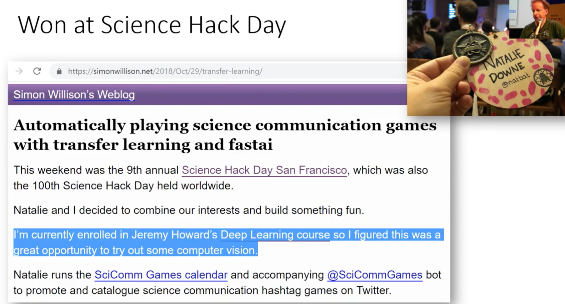
Simon Willison and Natalie Downe won a science hack day by creating twitter bot to identify #cougarOrNot pictures. I found it a very interesting project. Here is the blog and notebook. They used dataset from iNaturalist.

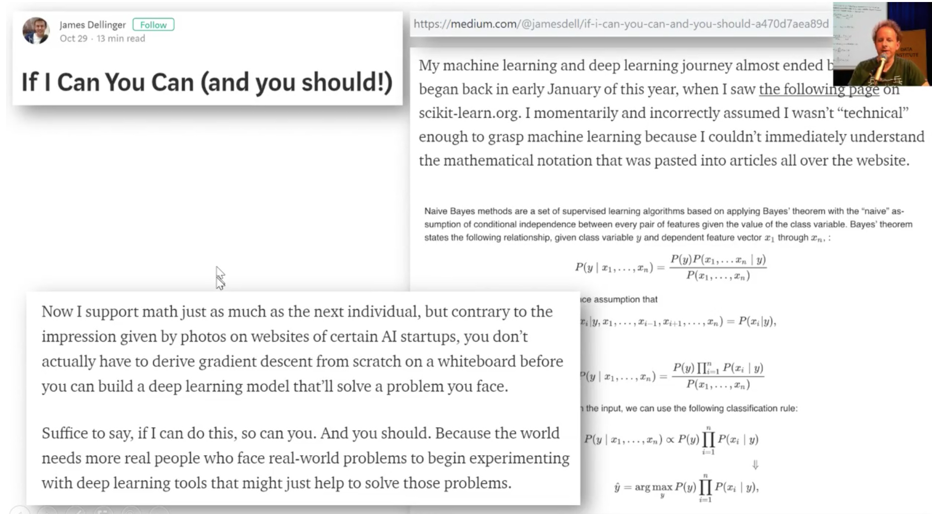
James Dellinger created a bird classifier and wrote in a blog post on the medium that he nearly didn’t start on deep learning at all. Because he went on scikit-learn.org and he saw these mathematical equations which were very difficult to understand fro a non-math person. But then because of fastai, he believed again that he can do deep learning without all this.

This is motivating. Daniel Armstrong on the forum started with not knowing anything to submit a PR to the library and getting that PR accepted.

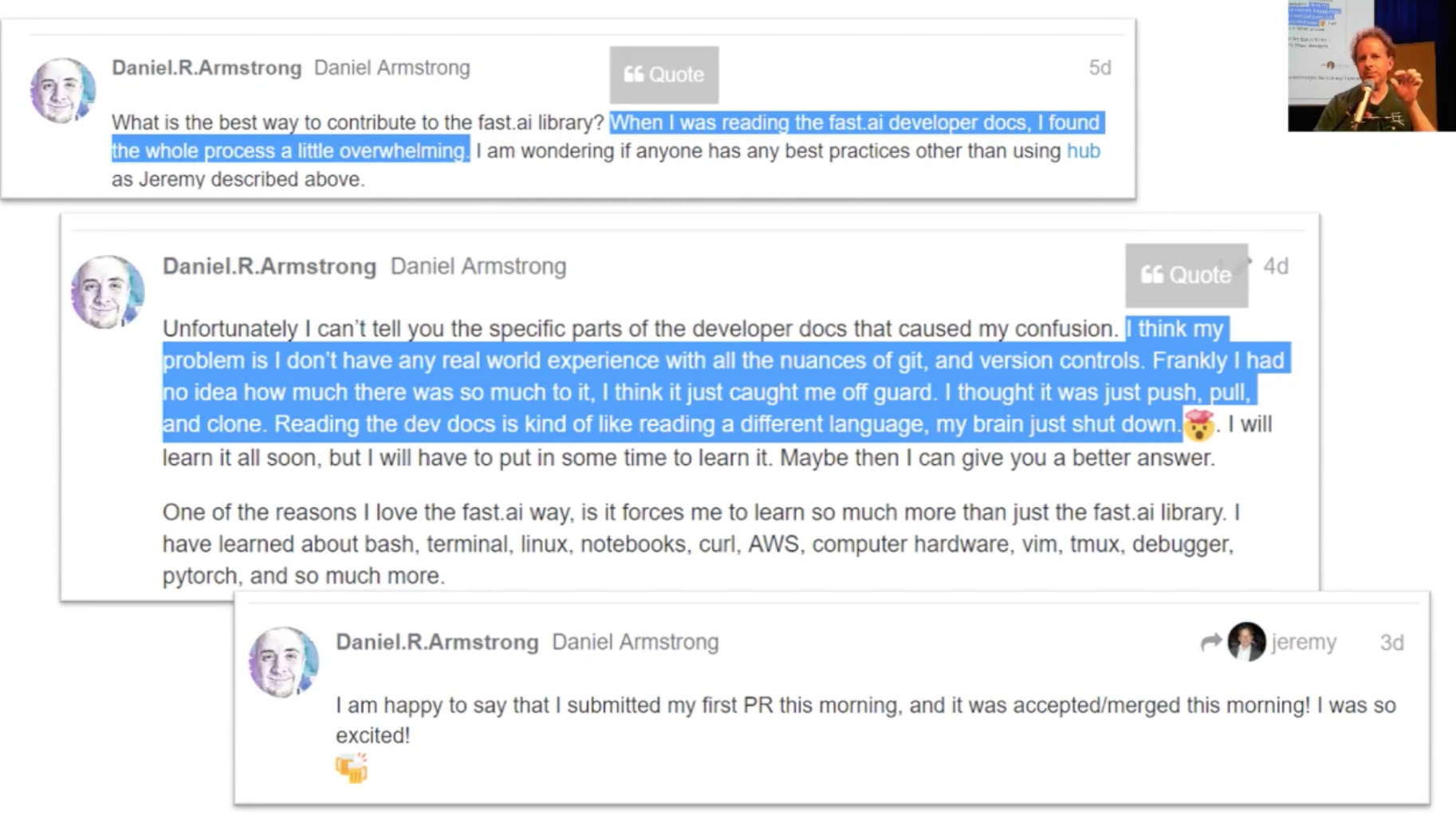
Advice: It’s ok to not know things. It ok to be intimidated. Just pick one small thing and begin with that. Push a small piece of code or documentation update or create a classifier.

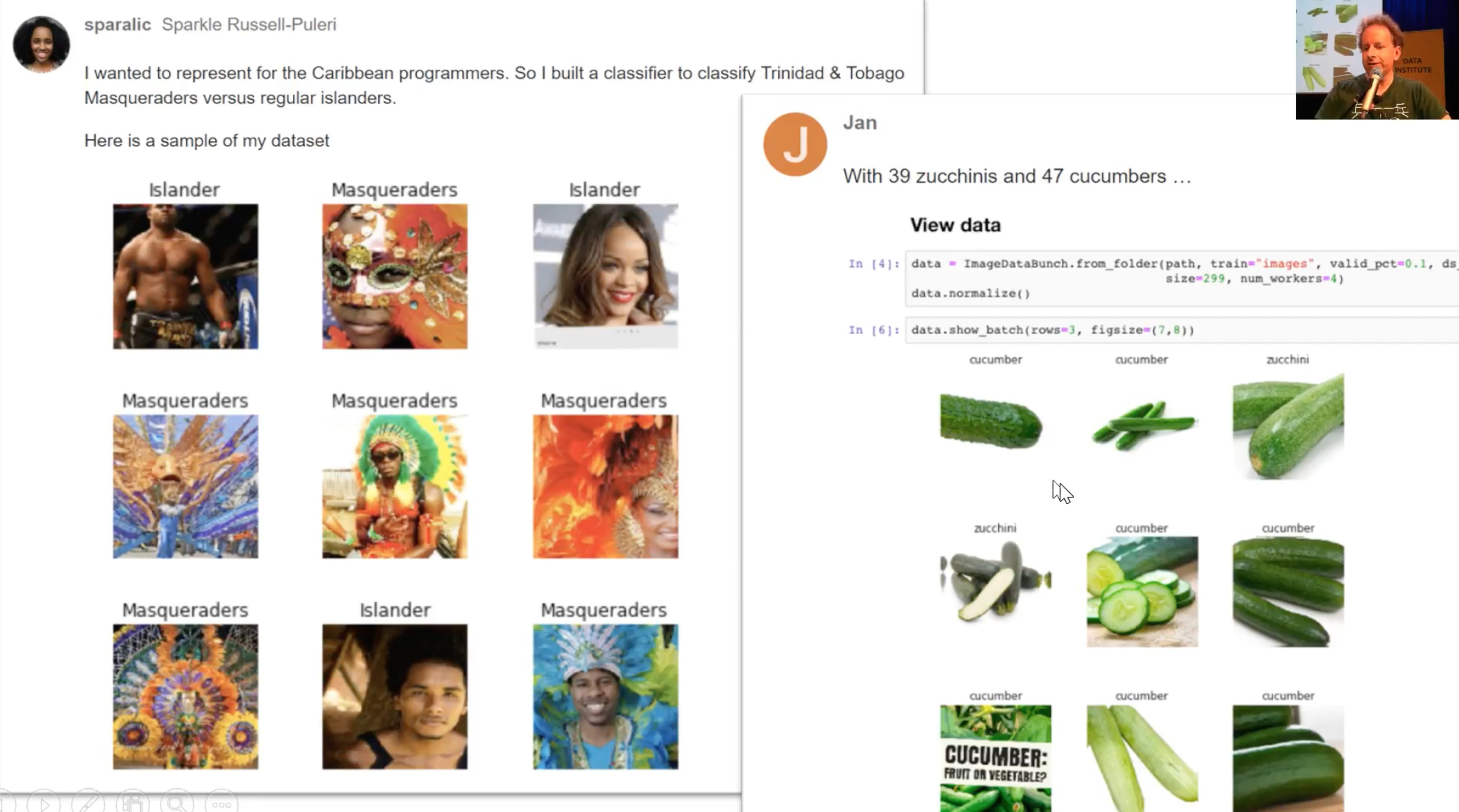
Some more classifiers on zucchini and cucumber images and classifying Trinidad and Tobago Musquredas.

This one takes dog and cat breeds model to discover what the main features are using the PCA technique.
Here is 1 feature related to body hair.

Anime classifier main feature seems hair color.

We can now detect the new buses over old ones in Panama city.

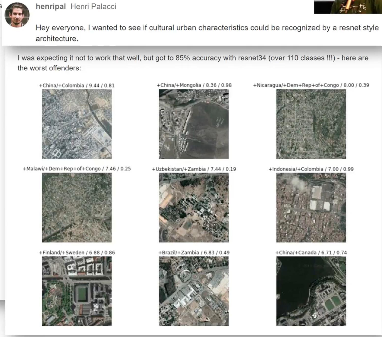
Which of the 110 countries a satellite image belongs to?
It must be beyond human performance.

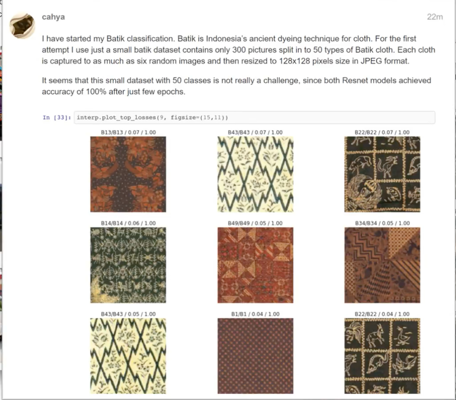
Batik cloth classification with 100% accuracy.

David went little further to recognize complete, incomplete and foundation buildings and plot them on the aerial satellite view.

Lots of fascinating projects It’s 1 week. It doesn’t mean you have to put your project out yet. Most of the people who created these projects have attended the previous course. That could have been a bit of head start.
But we will see today, how can you create your own classifier this week.

Next Steps

[12:57]

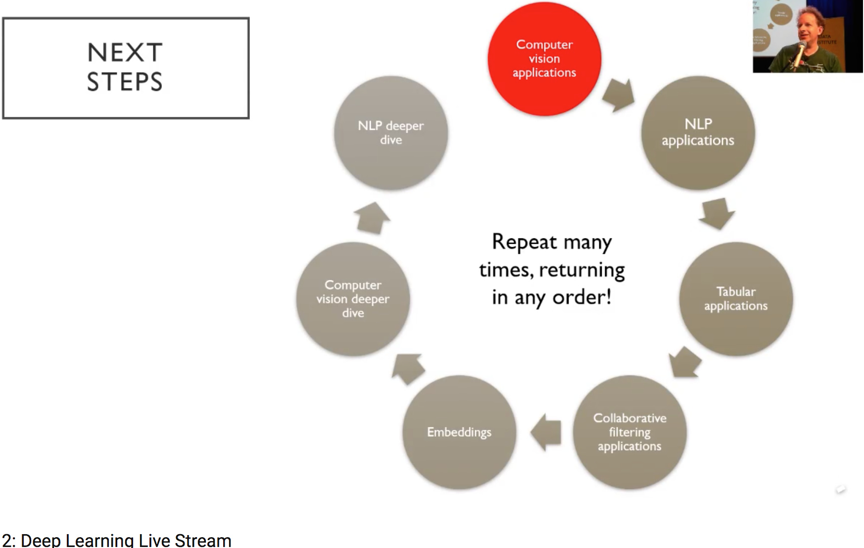
Let’s read this clockwise.
We will dig deeper into how to make these computer vision applications work well.
We will then look at the same thing for text and for tabular data, which is more like spreadsheets and databases. Then we will look at collaborative filtering which is for recommendations. That would take us to embeddings which is basically key underlying platforms behind these applications. That will take us back into more computer vision and more NLP.

What if you are stuck

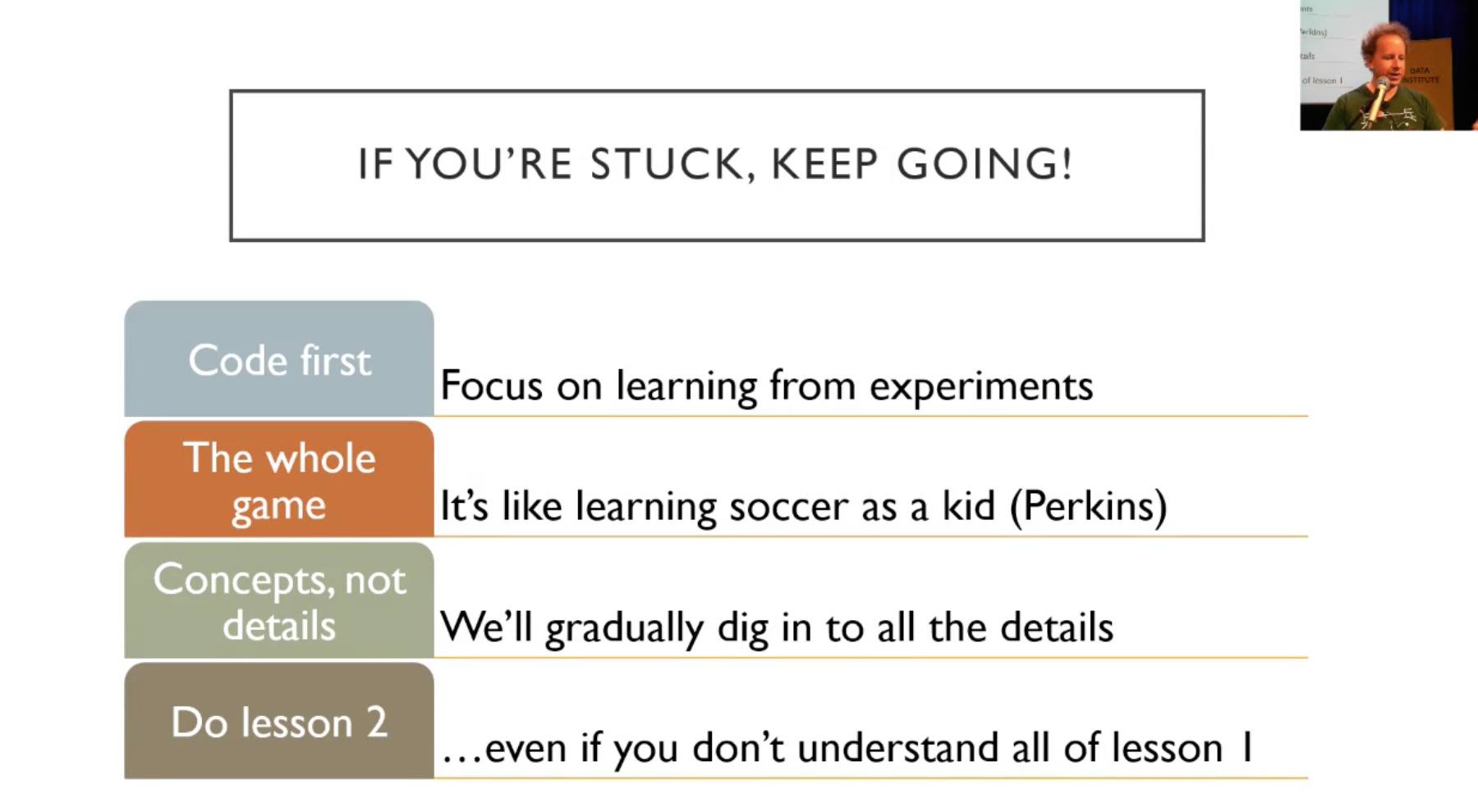
For those of people having a hard science background, in particular, go with code first approach. ‘Here is the code, type it in, start running it’ approach rather than here’s lots of theory approach, which is confusing, surprising and odd. Remember this basic tip - KEEP GOING.

You are not expected to understand everything yet. You are not expected to understand why everything works yet. you just wanna be in a situation where you enter the code, you can run it and get something happening and do experiments. and get a feel of what’s going on.

Most of the people who have got successful have watched videos at least 3 times. So don’t stop into lesson1, continue to 2, 3 and so on.
Rachel says, going over lessons 1 to 7 again and again even if you don’t understand things from previous lectures consistently continuing over next ones will clarify a lot of things gradually.

So this approach is based on a lot of academic research into learning theory and one person in particular David Perkins from Harvard has a great analogy of a kid learning to play the soccer game. He describes the approach of the whole game. If you are teaching a lid to play soccer, you don’t teach them how the friction between the ball and grass works. and teach them maths of how to kick the ball in the air etc. NO! you say here is the ball and watch some people playing soccer and now we’ll play soccer. and then the kid gradually over the following years learn to play soccer and get more and better at it.

This is what we’re trying to get you to do is to play soccer. Just type code, look at the inputs and see results.

Let’s dig into our first notebook today.

How to create your own Image dataset from google

[16:25]

lesson2-download.ipynb

You can create classifier with your own images. It will be all like last week’s pet detector but with your own images, you like.

How would you create your own classifier from scratch?

So, this approach is inspired by Adrian Rosebrock. who has his own website called pyimagesearch.

To distinguish between teddy bears, grizzly bears, and black bears.

Step 1:

Go to images.google.com
Search the category you want to download images of.
Press Ctrl+shift+j to pop up javascript console (Cmd+option+j for Mac)
Type this in the console

urls=Array.from(document.querySelectorAll(’.rg_i’)).map(el=> el.hasAttribute(‘data-src’)?el.getAttribute(‘data-src’):el.getAttribute(‘data-iurl’));
window.open(‘data:text/csv;charset=utf-8,’ + escape(urls.join(’\n’)));

This is a javascript code. Hit enter key.

It will pop up download box, choose the directory you want to save, type name of the text file and hit enter.
It will save all URLs of images you chose to download later in the text file on your computer.

Note this step has to be followed for each category you want to download images of.

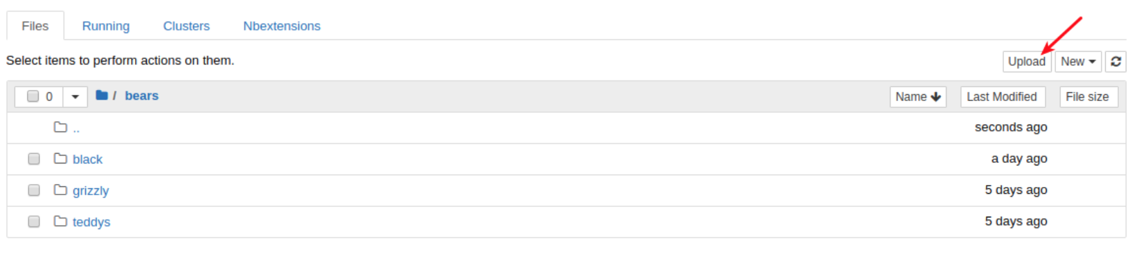
Step 2:

We need to get this text file uploaded on the server.
Remember when we are running our code in the Jupyter notebook, it’s running on one of the cloud providers, like Sagemaker, google cloud etc.

Let’s grab fastai library first.

from fastai import *
from fastai.vision import *

Let’s now create folders for each of the categories we want to classify.

folder = 'black' 
file = 'urls_black.txt'

folder = 'teddys'
file = 'urls_teddys.txt'

folder = 'grizzly' 
file = 'urls_grizzly.txt'

These are 3 cells doing the same things but with different information.
This is not reproducible research. This is something scientific background people horrified of.
We will create the folder named 'black and file named ‘urls_black.txt’.
Make sure this is the same name you have given to text file, you have saved your image URLs in.
Similar to other categories.

Then we have to run below cell to actually create those folders in the filesystem.

path = Path('data/bears')
dest = path/folder
dest.mkdir(parents=True, exist_ok=True)

You have to run black bear cell and skip next two and run mkdir cell(above code).
After that teddy cell and then mkdir cell and so on.

classes = ['teddys','grizzly','black']

download_images(path/file, dest, max_pics=200)

This will start downloading all images to your server.
Sometimes it might fail. It is running multiple processes in the background.
So error might not be clear.
Uncomment below section to set max_workers=0 if things don’t work out.

# If you have problems download, try with `max_workers=0` to see exceptions:
# download_images(path/file, dest, max_pics=20, max_workers=0)

Step 3:

for c in classes:
    print(c)
    verify_images(path/c, delete=True, max_workers=8)

Sometimes you might get corrupted images or the ones which are not in the required format.
If you set delete=True it will give you a clean dataset.

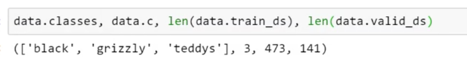
Step 4: Create ImageDataBunch

Now we have the basic structure to start Deep Learning.
When you download dataset from Kaggle or academic paper, there will be always folders called train, valid and test. In our case, we don’t have valid data, since we grabbed these images from Google search.
You definitely need a validation set, otherwise, you won’t know how well is your model going.

Whenever you create a data bunch, if you don’t have a separate training and validation set, then you can current folder. a simple . dot symbol says you intended directory is the current directory.
and We will set aside 20% of the data. So this is going to create a validation set for you automatically and randomly. You’ll see that whenever I create a validation set randomly, I always set my random seed to something fixed beforehand. This means that every time I run this code, I’ll get the same validation set. It is important is that you always have the same validation set. When you do hyperparameter tuning you need to have same valid set to decide which hyperparameter has improved metric.

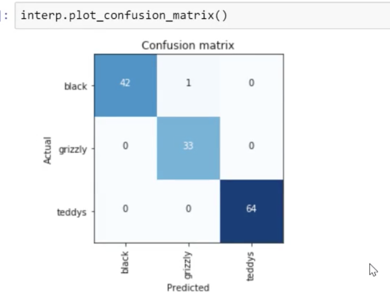
Classification Interpretation

1 black bear is misclassified.

Cleaning up:

Some of the top losses are bad but not because of our model but because of bad data. Sometimes, there are images in our dataset that do not relate to any of the data classes and shouldn’t be there.
Using the ImageCleaner widget from fastai.widgets we can prune our top losses, removing photos that don’t belong to any of the classes.

Step 1:

Import the required library

from fastai.widgets import *

Step 2:

Create a new Imagelist dataset without split for dataset cleaning. The loss will be calculated on every image and we can delete the images which are bad images and ultimately cleaning the dataset.

data = (ImageList.from_folder(path).split_none().label_from_folder().transform(size=224).databunch())

Please note, here we deliberately did not create a validation set. The idea is to run the ImageCleaner on the whole dataset train+validation.

Step 3:

Create a new CNN learner with the above new created databunch and load the model’s weights that you previously saved before these cleaning steps.

learn_clean = create_cnn(data, models.resnet34, metrics=error_rate)
learn_clean.load('Lesson 2 stage-2')

Step 4:

Calculate the losses

losses, idxs = DatasetFormatter().from_toplosses(learn_clean)

Step 5:

Run the image cleaner

ImageCleaner(losses, idxs, path)

It will display a widget, in which images, as well as their classes, will be displayed. You can select the images you want to remove from the dataset. The idea is to delete the images which are not unrelated to any of the classes. Click on Next Batch to see a new set of images, select the one you want to remove.
Notice that the widget will not delete images directly from disk but it will create a new CSV file cleaned.csv from where you can create a new ImageDataBunch with the corrected labels to continue training your model.

Step 6:

Create new databunch using the ‘cleaned.csv’ and train a model using it.

data_cleaned = ImageDataBunch.from_csv(path, csv_labels='cleaned.csv',
                                       label_col=1,
                                       valid_pct=0.2,
                                       ds_tfms=get_transforms(), size=224, 
                                       num_workers=0).normalize(imagenet_stats)

Put your model in production

Steps to export the content of our learned model and use it in production:

Step 1:

Export the model.

learn.export()

This will create a file named ‘export.pkl’ in the directory where we are working. The file contains everything we need to deploy our model (the model, the weights but also some metadata like the classes or the transforms/normalization used).

Optional step:

When we want to use CPU for prediction in the production environment:
Set fast.default.device to CPU

defaults.device = torch.device('cpu')

If you don’t have a GPU that happens automatically.

Step 2:

Open the image which is to be tested.

img = open_image(path/'filename.jpg')

ImageDataBunch.single_from_classes()

create_cnn()

Step-3:

Load the learner that we exported previously and predict the class of the img image file

learn = load_learner(path)
pred_class, pred_idx, outputs = learn.predict(img)`

the pred_class is the predicted class of the image, the outputs variable contains the probability of each of the classes. path is the path where your export.pkl file lies.

Homework - Give a try to a web app

Create a web app.

What can go wrong

Let’s look into some problems. The problems basically will be either

Your learning rate is too high or low
Your number of epochs
Try a few things:

1. Learning rate (LR) too high.

Let’s go back to our Teddy bear detector. and let’s make our learning rate really high. The default learning rate is 0.003 that works most of the time. So what if we try a learning rate of 0.5. That’s huge. What happens?

learn = create_cnn(data, models.resnet34, metrics=error_rate)

learn.fit_one_cycle(1, max_lr=0.5)

Total time: 00:13
epoch  train_loss  valid_loss  error_rate       
1      12.220007   1144188288.000000  0.765957    (00:13)

Our validation loss gets pretty damn high. Remember, this is something that’s normally something underneath 1. So if you see your validation loss do that, before we even learn what validation loss is, just know this, if it does that, your learning rate is too high. That’s all you need to know. Make it lower. Doesn’t matter how many epochs you do. If this happens, there’s no way to undo this. You have to go back and create your neural net again and fit from scratch with a lower learning rate.

2. Learning rate (LR) too low

What if we used a learning rate, not of default 0.003 but 1e-5 (0.00001)?

learn = create_cnn(data, models.resnet34, metrics=error_rate)

Previously we had this result:

Total time: 00:57
epoch  train_loss  valid_loss  error_rate
1      1.030236    0.179226    0.028369    (00:14)
2      0.561508    0.055464    0.014184    (00:13)
3      0.396103    0.053801    0.014184    (00:13)
4      0.316883    0.050197    0.021277    (00:15)

with learning rate =1e-5 we get

learn.fit_one_cycle(5, max_lr=1e-5)
Total time: 01:07
epoch  train_loss  valid_loss  error_rate
1      1.349151    1.062807    0.609929    (00:13)
2      1.373262    1.045115    0.546099    (00:13)
3      1.346169    1.006288    0.468085    (00:13)
4      1.334486    0.978713    0.453901    (00:13)
5      1.320978    0.978108    0.446809    (00:13)

And within one epoch, we were down to a 2 or 3% error rate.
With this really low learning rate, our error rate does get better but very very slowly.

We can plot it. So learn.recorder is an object which is going to keep track of lots of things happening while you train. You can call plot_losses to plot out the validation and training loss.

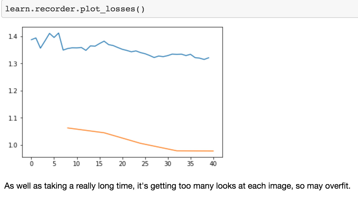
You can just see them gradually going down so slow. If you see that happening, then you have a learning rate which is too small. So bump it by 10 or bump it up by 100 and try again. The other thing you see if your learning rate is too small is that your training loss will be higher than your validation loss. You never want a model where your training loss is higher than your validation loss. That always means you haven’t fitted enough which means either your learning rate is too low or your number of epochs is too low. So if you have a model like that, train it some more or train it with a higher learning rate.

3. Too few epochs

learn = create_cnn(data, models.resnet34, metrics=error_rate, pretrained=False)

learn.fit_one_cycle(1)
Total time: 00:14
epoch  train_loss  valid_loss  error_rate
1      0.602823    0.119616    0.049645    (00:14)

What if we train for just one epoch? Our error rate is certainly better than random, 5%. But look at the difference between training loss and validation loss, a training loss is much higher than the validation loss. So too few epochs and too lower learning rate look very similar. So you can just try running more epochs and if it’s taking forever, you can try a higher learning rate. If you try a higher learning rate and the loss goes off to 100,000 million, then put it back to where it was and try a few more epochs. That’s the balance. That’s all you care about 99% of the time. And this is only the 1 in 20 times that the defaults don’t work for you.

4. Too many epochs

Too many epochs create something called overfitting". If you train for too long as we’re going to learn about it, it will learn to recognize your particular teddy bears but not teddy bears in general. Here is the thing. Despite what you may have heard, it’s very hard to overfit with deep learning. So we were trying today to show you an example of overfitting and Jeremy turned off everything. He turned off all the data augmentation, dropout, and weight decay. He tried to make it overfit as much as he can. He trained it on a small-ish learning rate and trained it for a really long time. And maybe he started to get it to overfit. Maybe.

np.random.seed(42)

data = ImageDataBunch.from_folder(path, train=".", valid_pct=0.9, bs=32, 
        ds_tfms=get_transforms(do_flip=False, max_rotate=0, max_zoom=1, max_lighting=0, max_warp=0
                              ),size=224, num_workers=4).normalize(imagenet_stats)
 
learn = create_cnn(data, models.resnet50, metrics=error_rate, ps=0, wd=0)
learn.unfreeze()

learn.fit_one_cycle(40, slice(1e-6,1e-4))

Total time: 06:39
epoch  train_loss  valid_loss  error_rate
1      1.513021    1.041628    0.507326    (00:13)
2      1.290093    0.994758    0.443223    (00:09)
3      1.185764    0.936145    0.410256    (00:09)
4      1.117229    0.838402    0.322344    (00:09)
5      1.022635    0.734872    0.252747    (00:09)
6      0.951374    0.627288    0.192308    (00:10)
7      0.916111    0.558621    0.184982    (00:09)
8      0.839068    0.503755    0.177656    (00:09)
9      0.749610    0.433475    0.144689    (00:09)
10     0.678583    0.367560    0.124542    (00:09)
11     0.615280    0.327029    0.100733    (00:10)
12     0.558776    0.298989    0.095238    (00:09)
13     0.518109    0.266998    0.084249    (00:09)
14     0.476290    0.257858    0.084249    (00:09)
15     0.436865    0.227299    0.067766    (00:09)
16     0.457189    0.236593    0.078755    (00:10)
17     0.420905    0.240185    0.080586    (00:10)
18     0.395686    0.255465    0.082418    (00:09)
19     0.373232    0.263469    0.080586    (00:09)
20     0.348988    0.258300    0.080586    (00:10)
21     0.324616    0.261346    0.080586    (00:09)
22     0.311310    0.236431    0.071429    (00:09)
23     0.328342    0.245841    0.069597    (00:10)
24     0.306411    0.235111    0.064103    (00:10)
25     0.289134    0.227465    0.069597    (00:09)
26     0.284814    0.226022    0.064103    (00:09)
27     0.268398    0.222791    0.067766    (00:09)
28     0.255431    0.227751    0.073260    (00:10)
29     0.240742    0.235949    0.071429    (00:09)
30     0.227140    0.225221    0.075092    (00:09)
31     0.213877    0.214789    0.069597    (00:09)
32     0.201631    0.209382    0.062271    (00:10)
33     0.189988    0.210684    0.065934    (00:09)
34     0.181293    0.214666    0.073260    (00:09)
35     0.184095    0.222575    0.073260    (00:09)
36     0.194615    0.229198    0.076923    (00:10)
37     0.186165    0.218206    0.075092    (00:09)
38     0.176623    0.207198    0.062271    (00:10)
39     0.166854    0.207256    0.065934    (00:10)
40     0.162692    0.206044    0.062271    (00:09)

Basically, if you are overfitting there is only one thing you can notice which is that the error rate improves for a while and then starts getting worse again. You will see a lot of people, even people that claim to understand machine learning, tell you that if your training loss is lower than your validation loss, then you are overfitting. As you will learn today in more detail and during the rest, of course, that is absolutely not true.
Any model that is trained correctly will always have train loss lower than validation loss.
That is not a sign of overfitting. That is not a sign you’ve done something wrong. That is a sign you have done something right. The sign that you’re overfitting is that your error starts getting worse because that’s what you care about. You want your model to have a low error. So as long as you’re training and your model error is improving, you’re not overfitting. How could you be?

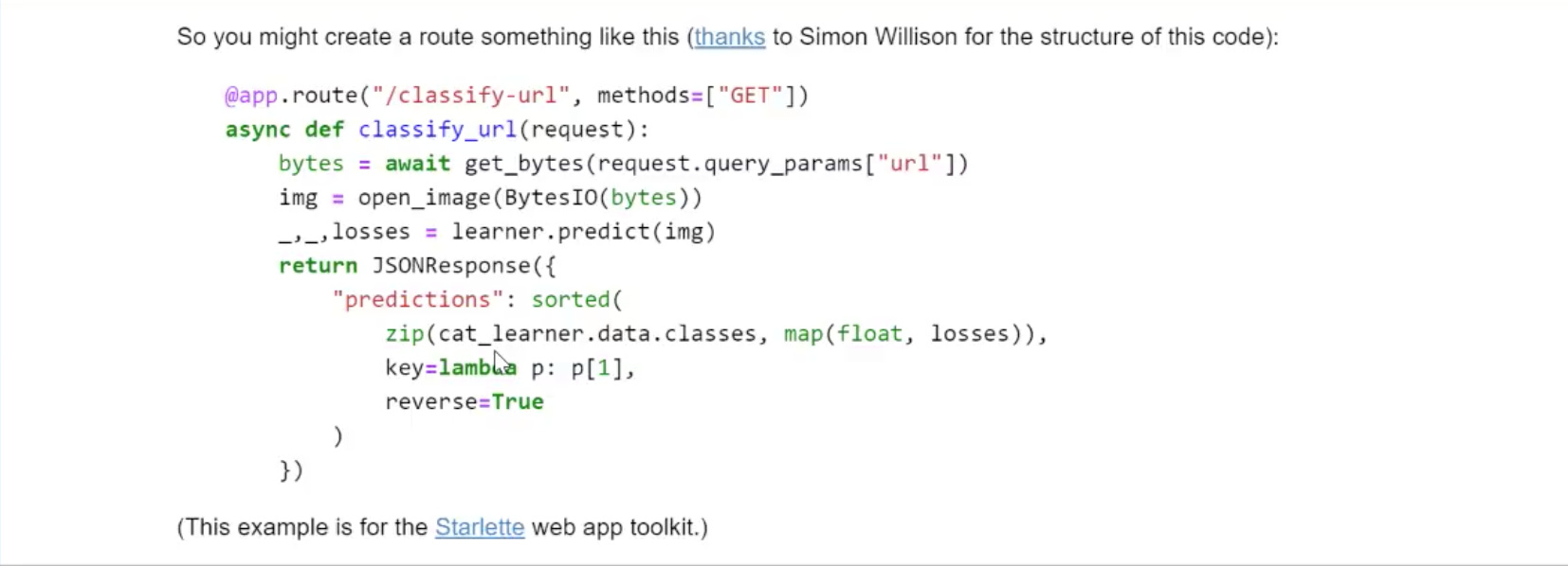
Conclusion:

So these are the main 4 things that can go wrong. There are some other details that we will learn about during the rest of this course but honestly if you stopped listening now (please don’t, that would be embarrassing) and you’re just like okay I’m going to go and download images, I’m going to create CNN with resnet34 or resnet50, I’m going to make sure that my learning rate and number of epochs is okay and then I’m going to chuck them up in a Starlette web API, most of the time you are done. At least for computer vision. Hopefully, you will stick around because you want to learn about NLP, collaborative filtering, tabular data, and segmentation, etc as well.

Mathematics behind predictions, losses

Let’s now understand what’s actually going on. What does “loss” or “epoch” or “learning rate” mean? Because for you to really understand these ideas, you need to know what’s going on. So we are going to go all the way to the other side. Rather than creating a state of the art cougar detector, we’re going to go back and create the simplest possible linear model. So we’re going to actually see a little bit of math. But don’t be turned off. It’s okay. We’re going to do a little bit of math but it’s going to be totally fine. Even if math is not your thing.
Because the first thing we’re going to realize is that when we see a picture like this number eight.

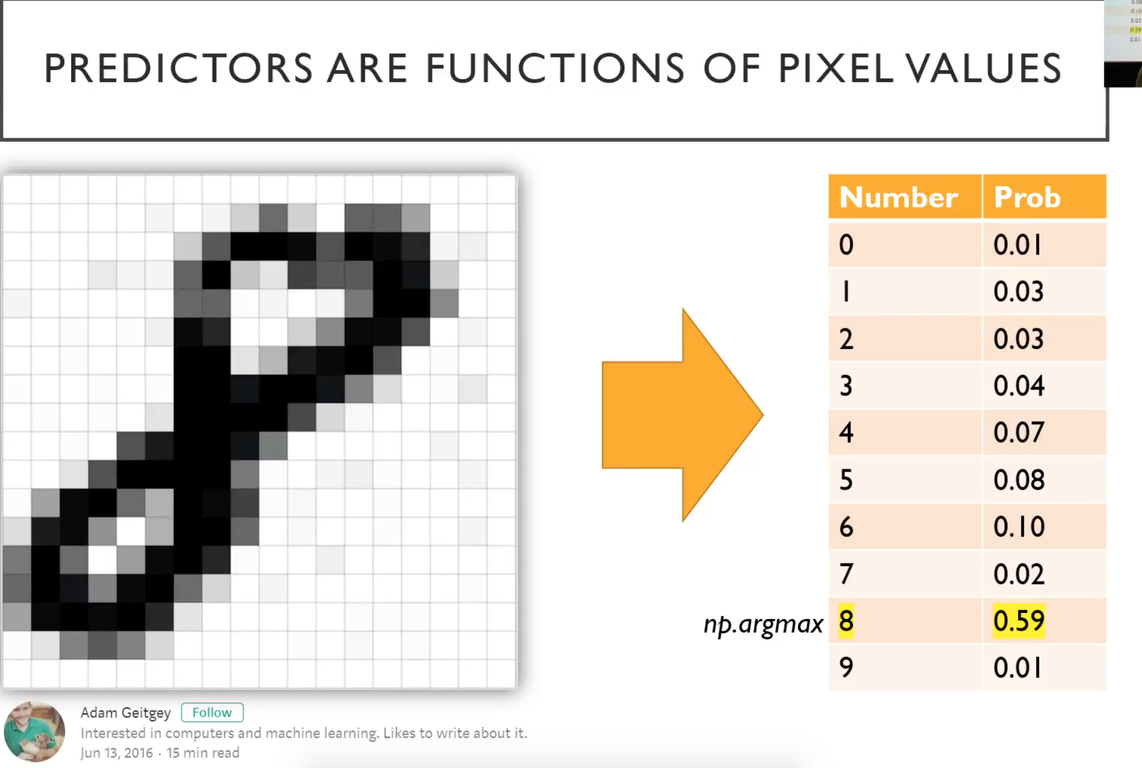
It’s actually just a bunch of numbers. For this grayscale one, it’s a matrix of numbers. If it was a color image, it would have a third dimension. So when you add an extra dimension, we call it a tensor rather than a matrix. It would be a 3D tensor of numbers ﹣ red, green, and blue.

When we created that teddy bear detector, what we actually did was we created a mathematical function that took the numbers from the images of the teddy bears and a mathematical function converted those numbers into, in our case, three numbers: a number for the probability that it’s a teddy, a probability that it’s a grizzly, and the probability that it’s a black bear. In this case, there’s some hypothetical function that’s taking the pixel representing a handwritten digit and returning ten numbers: the probability for each possible outcome (i.e. the numbers from zero to nine).

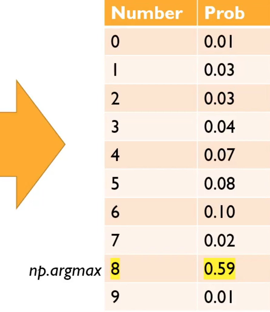
What you’ll often see in our code and other deep learning code is that you’ll find this bunch of probabilities and then you’ll find a function called max or argmax attached to it. What that function is doing is, it’s saying find the highest number (i.e. probability) and tell me what the index is.

np.argmax

or

torch.argmax

of the above array would return the index 8.

In fact, let’s try it. We know that the function to predict something is called learn.predict . So we can chuck two question marks before or after it to get the source code.

And here it is.

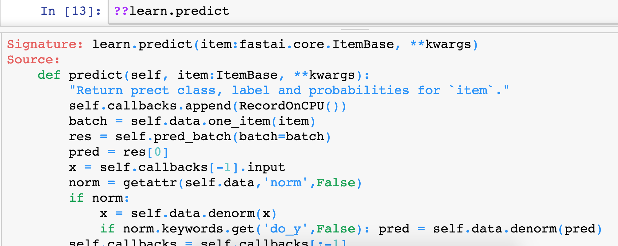
pred_max = res.argmax() . Then what is the class? We just pass that into the classes array. So you should find that the source code in the fastai library can both strengthen your understanding of the concepts and make sure that you know what’s going on and really help you here.

Question: Can we have a definition of the error rate being discussed and how it is calculated? I assume it’s cross-validation error [56:37].

Sure. So one way to answer the question of how is error rate calculated would be to type error_rate?? and look at the source code, and it’s 1 - accuracy.

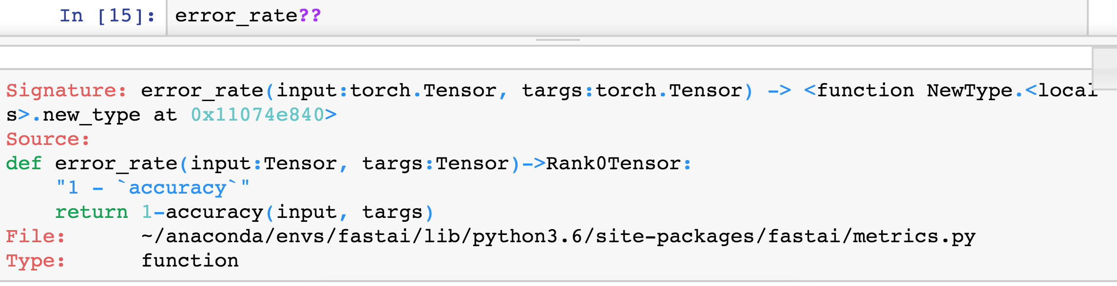
So then a question might be what is accuracy:

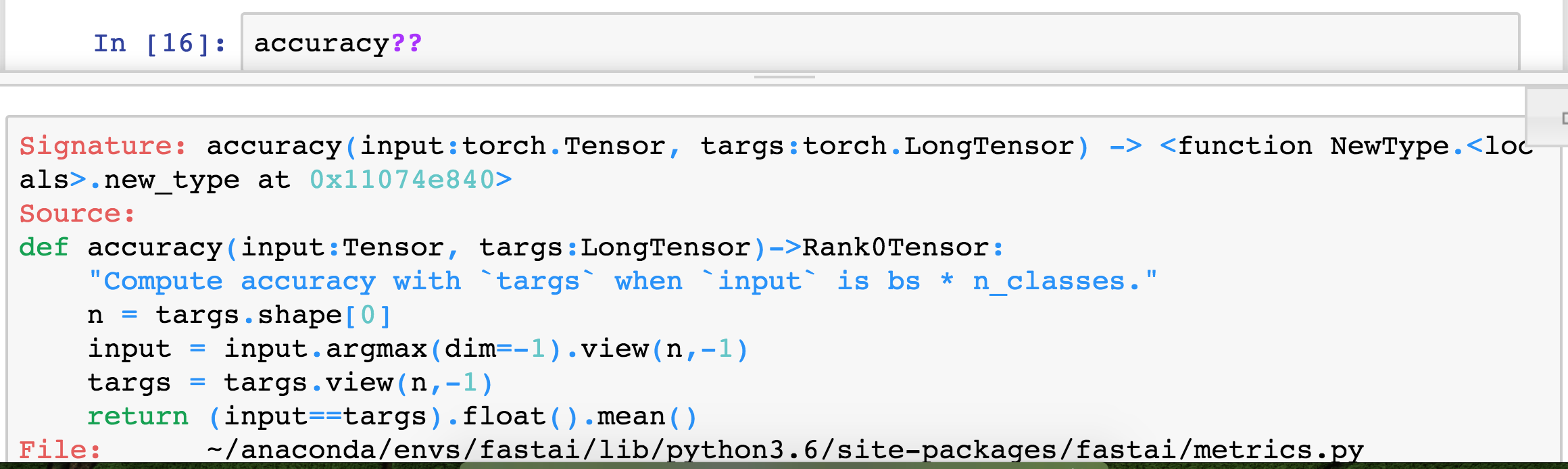
It is argmax. So we now know that means to find out which particular thing it is, and then look at how often that equals the target (i.e. the actual value) and take the mean. So that’s basically what it is. So then the question is, what does that being applied to and always in fastai, metrics (i.e. the things that we pass in) are always going to be applied to the validation set. Any time you put a metric here, it’ll be applied to the validation set because that’s your best practice.

learn = create_cnn(data, models.resnet50, metrics=error_rate, ps=0, wd=0)
learn.unfreeze()

learn.fit_one_cycle(40, slice(1e-6,1e-4))

Total time: 06:39
epoch  train_loss  valid_loss  error_rate
1      1.513021    1.041628    0.507326    (00:13)
2      1.290093    0.994758    0.443223    (00:09)
3      1.185764    0.936145    0.410256    (00:09)
4      1.117229    0.838402    0.322344    (00:09)
5      1.022635    0.734872    0.252747    (00:09)
6      0.951374    0.627288    0.192308    (00:10)
7      0.916111    0.558621    0.184982    (00:09)

That’s what you always want to do is make sure that you’re checking your performance on data that your model hasn’t seen, and we’ll be learning more about the validation set shortly.

Remember, you can also type doc() if the source code is not what you want which might well not be, you actually want the documentation, that will both give you a summary of the types in and out of the function and a link to the full documentation where you can find out all about how metrics work and what other metrics there are and so forth. Generally speaking, you’ll also find links to more information where, for example, you will find a complete run through and sample code showing you how to use all these things. So don’t forget that the doc() function is your friend. Also both in the doc function and in the documentation, you’ll see a source link. This is like ?? but what the source link does is it takes you into the exact line of code in Github. So you can see exactly how that’s implemented and what else is around it. So lots of good stuff there.

Question: Why were you using 3e for your learning rates earlier? With 3e-5 and 3e-4

[59:10]

We found that 3e-3 is just a really good default learning rate. It works most of the time for your initial fine-tuning before you unfreeze. And then, I tend to kind of just multiply from there. So then the next stage, I will pick 10 times lower than that for the second part of the slice, and whatever the LR finder found for the first part of the slice. The second part of the slice doesn’t come from the LR finder. It’s just a rule of thumb which is 10 times less than your first part which defaults to 3e-3, and then the first part of the slice is what comes out of the LR finder. We’ll be learning a lot more about these learning rate details both today and in the coming lessons. But for now, all you need to remember is that your basic approach looks like this.

RULE OF THUMB

learn.fit_one_cycle(4, 3e-3) # num of epochs = 4, lr = 3e-3 default
learn.unfreeze()

learn.fit_one_cycle() takes number of epochs, Jeremy often picks 4
and learning rate which defaults to 3e-3. Let’s fit that for a while and then we unfreeze it.

learn.fit_one_cycle(4, slice(xxx, 3e-4))

Then we learn some more and so this time Jeremy takes previous learning rate finder value 3e-3 and divide it by 10 so 3e-4. Then he also writes a slice with another number and that’s the number he gets from the learning rate finder﹣a bit where it’s got the strongest slope.

THIS IS RULE OF THUMB WHICH WORKS MOST OF THE TIME.
Let’s dig in further to understand it more completely.

We’re going to create this mathematical function that takes the numbers that represent the pixels and spits out probabilities for each possible class.

By the way, a lot of the stuff that we’re using here, we are stealing from other people who are awesome and so we’re putting their details here. So please check out their work because they’ve got great work that we are highlighting in our course. Jeremy really likes this idea of this little-animated gif of the numbers, so thank you to Adam Geitgey for creating that.

Linear Regression Function [01:02:04]

Let’s look and see how we create one of these functions, and let’s start with the simplest functions Jeremy knows.

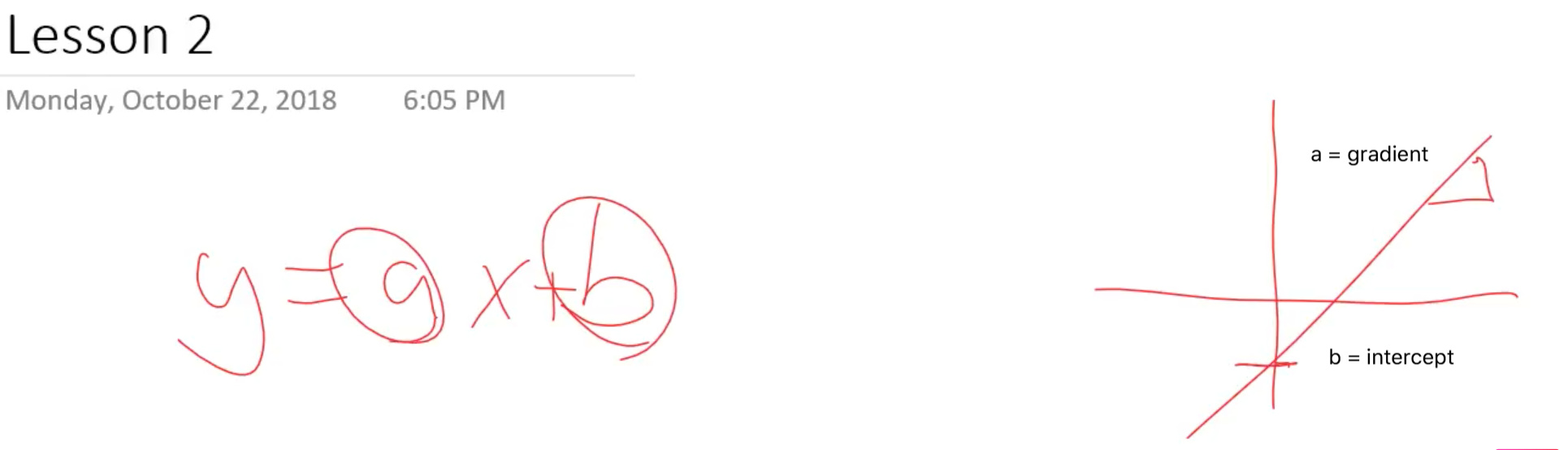
y = ax + b

That is a line where

a is a gradient of the line
b is the intercept of the line

Hopefully, when we said that you need to know high school math to do this course, these are the things we are assuming that you remember. If we do mention some math thing which Jeremy assuming you remember and you don’t remember it, don’t freak out. It happens to all of us. Khan Academy is actually terrific. It’s not just for school kids. Go to Khan Academy, find the concept you need a refresher on, and he explains things really well. So strongly recommend checking that out. Remember, Jeremy is just a philosophy student, so all the time he’s trying to either remind himself about something or he never learned something. So we have the whole internet to teach us these things.

So Jeremy rewrites equation slightly

y = a₁x+a₂

So let’s just replace ‘b’ with a₂, just give it a different name.

There’s another way of saying the same thing. Then another way of saying that would be if we could multiply a ₂ by number 1.

y = a₁x + a₂ . 1

This still is the same thing. Now at this point, Jeremy actually going to say let’s not put the number 1 there but put an are equivalent of 1 with a bit of renaming.

y = a₁ . x₁ + a₂ . x₂ [x₂ = 1]

So these 2 equations

y = ax + b

and

y = a₁ . x₁ + a₂ . x₂ [x₂ = 1]

are equivalent with little. bit of renaming

Now in machine learning, we don’t just have one equation, we’ve got lots.

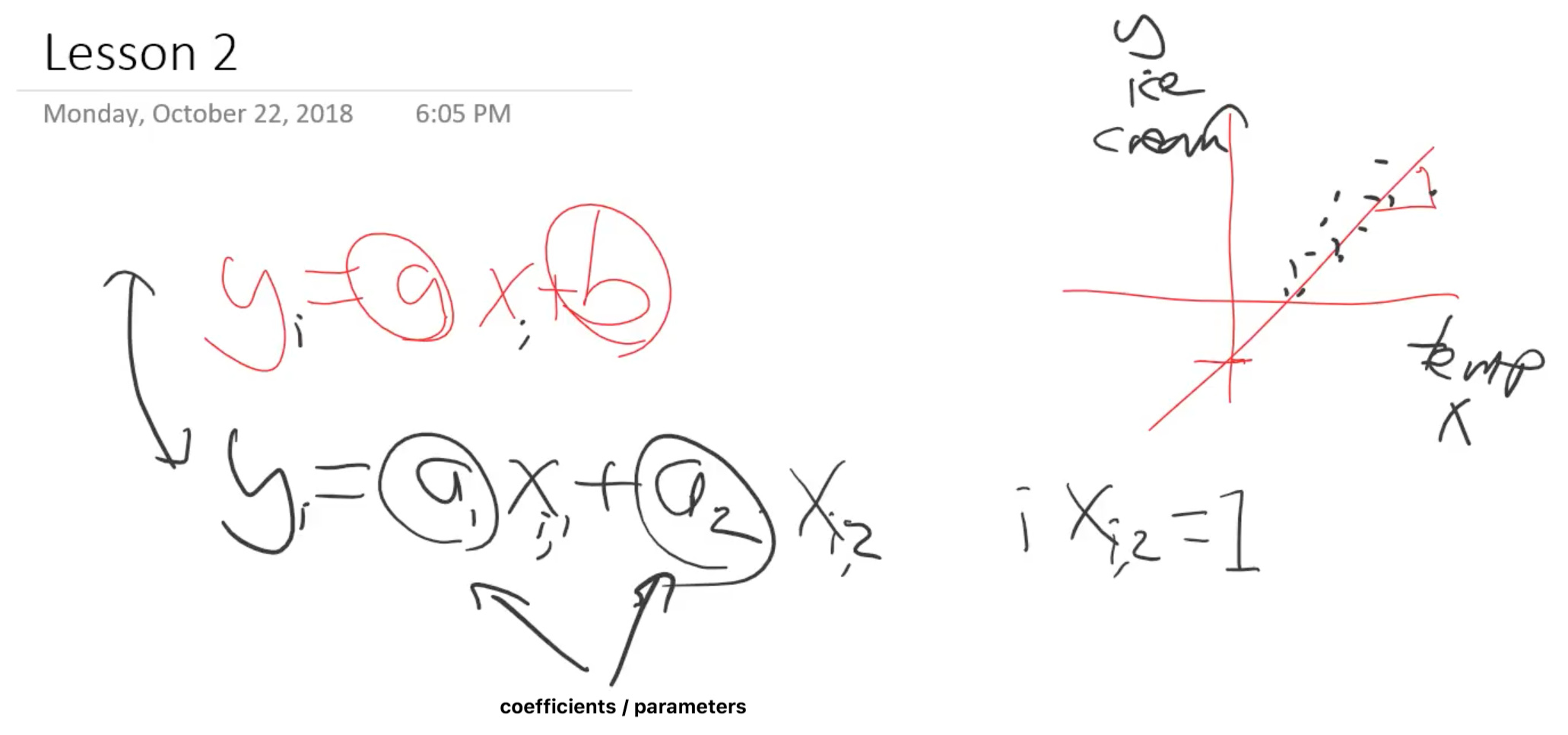
So if we’ve got some data that represents the temperature versus the number of ice creams sold, then we have lots of dots (data points).

So each one of these dots, we might hypothesize is based on this formula

y = a₁ . x₁ + a₂ . x₂

And basically, there are lots of values of y and lots of values of x so we can stick little subscript ‘i’ here.

y_i = ax_i + b

The way we do that is a lot like numpy indexing, but rather things in square brackets, we put them down here as the subscript in our equation.

y_i = a₁ . x_i,1 + a₂ . x_i,2

So this is now saying there’s actually lots of these different y_i’s based on lots of different x_i,1’s and x_i,2’s. But notice there is still one of each of these (a₁,a₂). They called the coefficients or the parameters.

So this is our linear equation and we are still going to say that every x₂ = 1

Why did Jeremy do it that way? Because he wants to do linear algebra? Why does he want to do in linear algebra? One reason is that Rachel teaches the world’s best linear algebra course, so if you’re interested, check it out. So it’s a good opportunity for Jeremy to throw in a pitch for this which they make no money but never mind. But more to the point right now, it’s going to make life much easier. Because Jeremy hates writing loops, he hates writing code. He just wants the computer to do everything for him. And anytime you see this little ‘i’ subscripts, that sounds like you’re going to have to do loops and all kind of stuff. But what you might remember from school is that when you’ve got two things being multiplied together and another two things being multiplied together, then they get added up, that’s called a “dot product”. If you do that for lots and lots of different numbers ‘i’, then that’s called a matrix product.

So in fact, this whole thing can be rewritten as:

\vec{y} = X \vec{a}

Rather than lots of different y_i’s we can say thta there is one vector called y which is equal to one matrix called X times one vector callled a.
At this point, Jeremy says a lot of you don’t remember that. That’s fine. We have a picture to show you.

Andre Staltz created this fantastic website called matrixmultiplication.xyz and here we have a matrix by a vector, and we are going to do a matrix-vector product.

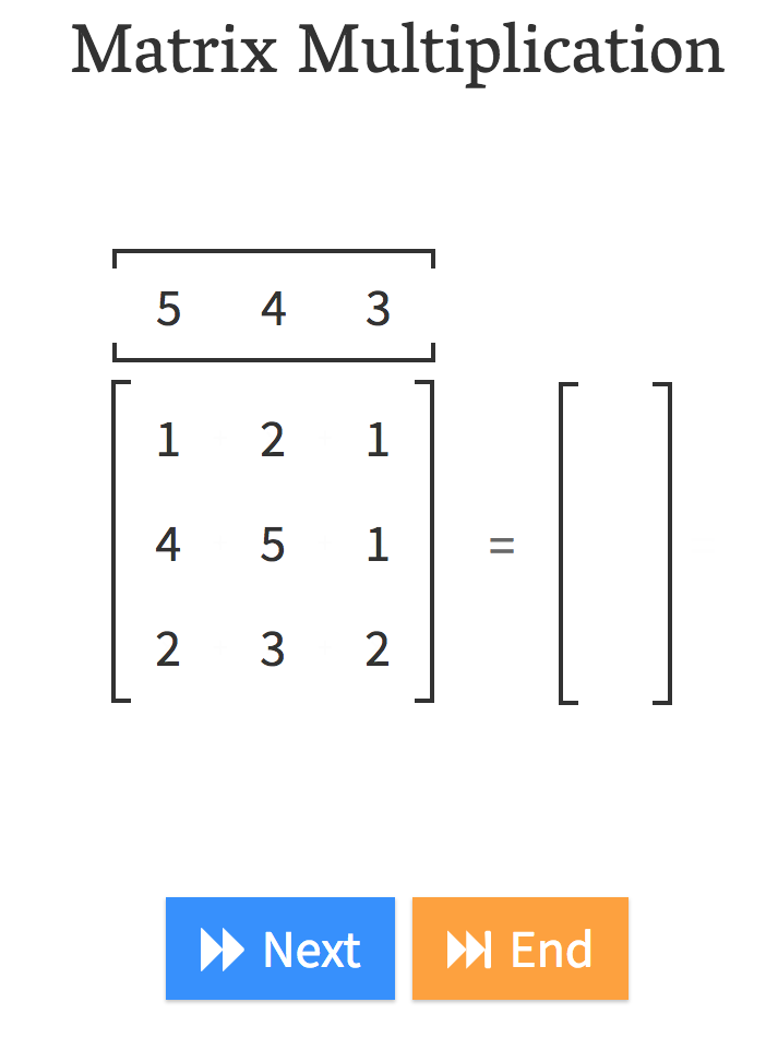
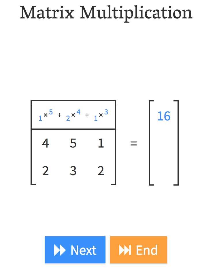
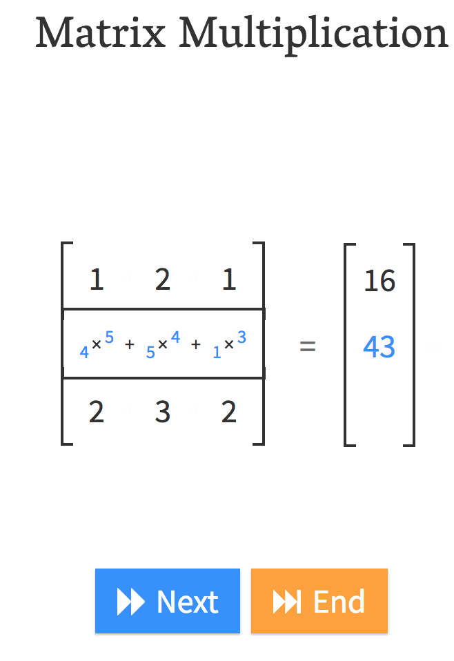
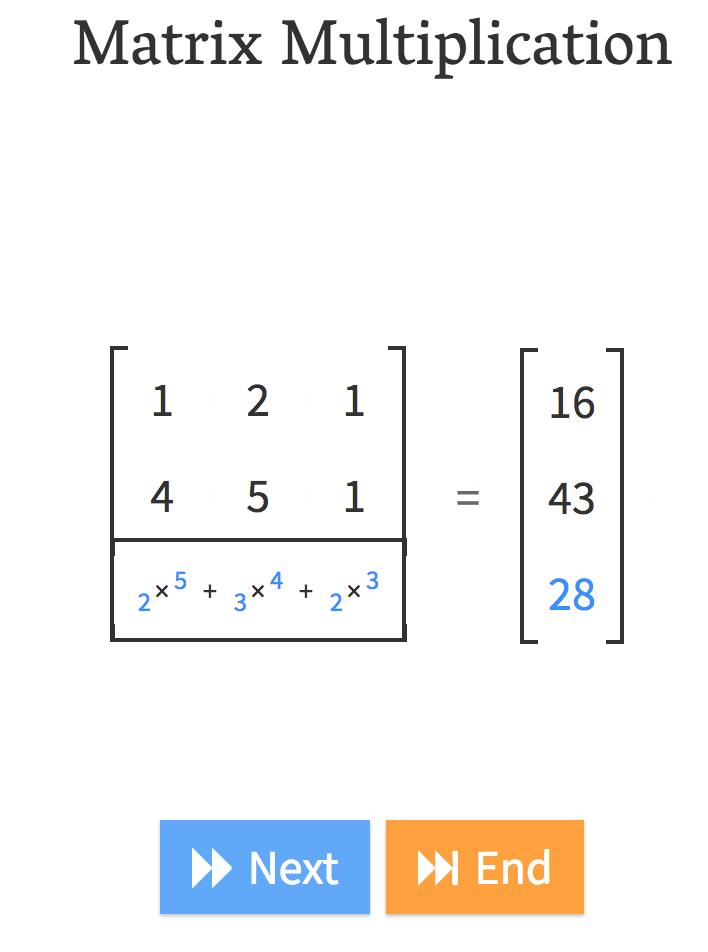
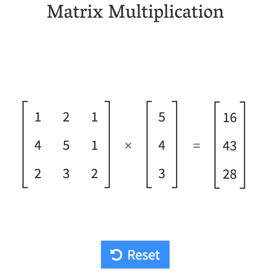
That is what matrix-vector multiplication does.

In other words, , it’s just
y_i = a₁ . x_i,1 + a₂ . x_i,2

Question: When generating new image dataset, how do you know how many images are enough? What are ways to measure “enough”? [01:08:36]

That’s a great question. Another possible problem you have is you don’t have enough data. How do you know if you don’t have enough data? Because you found a good learning rate (i.e. if you make it higher than it goes off into massive losses; if you make it lower, it goes really slowly) and then you train for such a long time that your error starts getting worse. So you know that you trained for long enough. And you’re still not happy with the accuracy﹣it’s not good enough for the teddy bear cuddling level of safety you want. So if that happens, there’s a number of things you can do and we’ll learn pretty much all of them during this course but one of the easiest one is get more data. If you get more data, then you can train for longer, get higher accuracy, lower error rate, without overfitting.

Unfortunately, there is no shortcut. I wish there was. I wish there’s some way to know ahead of time how much data you need. But I will say this﹣most of the time, you need less data than you think. So organizations very commonly spend too much time gathering data, getting more data than it turned out they actually needed. So get a small amount first and see how you go.

Question: What do you do if you have unbalanced classes such as 200 grizzly and 50 teddies? [1:10:00]

Nothing. Try it. It works. A lot of people ask this question about how do I deal with unbalanced data. I’ve done lots of analysis with unbalanced data over the last couple of years and I just can’t make it not work. It always works. There’s actually a paper that said if you want to get it slightly better then the best thing to do is to take that uncommon class and just make a few copies of it. That’s called “oversampling” but I haven’t found a situation in practice where I needed to do that. I’ve found it always just works fine, for me.

Question: Once you unfreeze and retrain with one cycle again if your training loss is still higher than your validation loss (likely underfitting), do you retrain it unfrozen again (which will technically be more than one cycle) or you redo everything with longer epoch per the cycle? [01:10:48]

You guys asked me that last week. My answer is still the same. I don’t know. Either is fine. If you do another cycle, then it’ll maybe generalize a little bit better. If you start again, do twice as long, it’s kind of annoying, depends how patient you are. It won’t make much difference. For Jeremy personally, he normally just trains a few more cycles. But it doesn’t make much difference most of the time.

Question

classes = ['black', 'grizzly', 'teddys']
data2 = ImageDataBunch.single_from_classes(path, classes, tfms=get_transforms(), size=224).normalize(imagenet_stats)
learn = create_cnn(data2, models.resnet34).load('stage-2')

This requires

models.resnet34

which I find surprising, I had assumed that the model created by .save(...) (which is about 85MB on disk) would be able to run without also needing a copy of resnet34??

We’re going to be learning all about this shortly. There is no “copy of ResNet34”, ResNet34 is what we call “architecture”﹣it’s a functional form. Just like

y = ax + b

is a linear functional form. It doesn’t take up any room, it doesn’t contain anything, it’s just a function. ResNet34 is just a function. I think the confusion here is that we often use a pre-trained neural net that’s been learned on ImageNet. In this case, we don’t need to use a pre-trained neural net. Actually, to avoid that even getting created, you can actually pass pretrained=False.

learn = create_cnn(data, models.resnet34, metrics=error_rate, pretrained=False)

That’ll ensure that nothing even gets loaded which will save you another 0.2 seconds, I guess. But we’ll be learning a lot more about this. So don’t worry if this is a bit unclear. The basic idea is models.resnet34 above is basically the equivalent of saying is it a line or is it a quadratic or is it a reciprocal﹣this is just a function. This is a ResNet34 function. It’s a mathematical function. It doesn’t take any storage, it doesn’t have any numbers, it doesn’t have to be loaded as opposed to a pre-trained model. When we did it at the inference time, the thing that took space is this bit

learn.load('stage-2')

Which is where we load our parameters. It is basically saying, as we about find out, what are the values of
a, b we have to store these numbers. But for ResNet 34, you don’t just store 2 numbers, you store a few million or few tens of millions of numbers.

[1:14:13 ]

So why did we do all this? It’s because we wanted to be able to write it out like this

\vec{y} = X \vec{a}
and the reason I wanted to be able to like this is that we can now do that in PyTorch with no loops, single line of code, and it’s also going to run faster. PyTorch really doesn’t like loops. It really wants you to send it a whole equation to do all at once. Which means, you really want to try and specify things in these kinds of linear algebra ways. So let’s go and take a look because what we’re going to try and do then is we’re going to try and take this

\vec{y} = X \vec{a}

We’re going to call this an architecture. It’s the world’s tiniest neural network. It’s got two parameters
a₁ and a₂. We are going to try and fit this architecture with some data.

Stochastic Gradient Descent (SGD) [1:15:06]

So let’s jump into a notebook and generate some dots, and see if we can get it to fit a line somehow. And the “somehow” is going to be using something called SGD. What is SGD? Well, there’s two types of SGD. The first one is where Jeremy said in lesson 1 “hey you should all try building these models and try and come up with something cool” and you guys all experimented and found the really good stuff. So that’s where the S would be Student. That would be Student Gradient Descent. So that’s version one of SGD.

Version two of SGD which is what Jeremy is going to talk about today is where we are going to have a computer try lots of things and try and come up with a really good function and that would be called Stochastic Gradient Descent. The other one that you hear a lot on Twitter is Stochastic Grad student Descent.

Linear regression problem 1:16:07

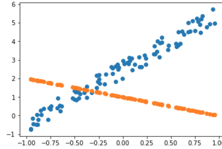
We are going to jump into lesson2-sgd.ipynb. We are going to go bottom-up rather than top-down. We are going to create the simplest possible model we can which is going to be a linear model. And the first thing we need is we need some data. So we are going to generate some data. The data we’re going to generate looks like this:

So x-axis might represent temperature, y-axis might represent the number of ice creams we sell or something like that. But we’re just going to create some synthetic data that we know is following a line. As we build this, we’re actually going to learn a little bit about PyTorch as well.

The goal of linear regression is to fit a line to a set of points.

n=100

x = torch.ones(n,2) 

x[:,0].uniform_(-1.,1)

x[:5]

tensor([[ 0.1695,  1.0000],
        [-0.3731,  1.0000],
        [ 0.4746,  1.0000],
        [ 0.7718,  1.0000],
        [ 0.5793,  1.0000]])

Basically the way we’re going to generate this data is by creating some coefficients a₁ will be 3 and a₂ will be 2. We are going to create a column of numbers for our x’s and a whole bunch of 1’s.

 a = tensor(3.,2); a
 tensor([3., 2.])

And then we’re going to do this x@a. What is x@a? x@a in Python means a matrix product between x and a. And it actually is even more general than that. It can be a vector-vector product, a matrix-vector product, a vector-matrix product, or a matrix-matrix product. Then actually in PyTorch, specifically, it can mean even more general things where we get into higher rank tensors which we will learn all about very soon. But this is basically the key thing that’s going to go on in all of our deep learning. The vast majority of the time, our computers are going to be basically doing this﹣multiplying numbers together and adding them up which is the surprisingly useful thing to do.

y = x@a + torch.rand(n)

So we basically are going to generate some data by creating a line and then we’re going to add some random numbers to it. But let’s go back and see how we created x and a. Jeremy mentioned that we’ve basically got these two coefficients 3 and 2. And you’ll see that we’ve wrapped it in this function called tensor(). You might have heard this word ‘tensor’ before. It’s one of these words that sounds scary and apparently if you’re a physicist, it actually is scary. But in the world of deep learning, it’s actually not scary at all. Tensor means array, but specifically, it’s an array of a regular shape. So it’s not an array where row 1 has two things, row 3 has three things, and row 4 has one thing, what you call a “jagged array”. That’s not a tensor. A tensor is an array which has a rectangular or cube or whatever ﹣ a shape where every row is the same length and every column is the same length. The following are all tensors -

A 4 by 3 matrix
A vector of length 4
A 3D array of length 3 by 4 by 6

That’s all tensor is. We have these all the time. For example, an image is a 3-dimensional tensor. It’s got a number of rows by a number of columns by a number of channels (normally red, green, blue). So for example, VGA picture could be 640 by 480 by 3 or actually we do things backward so when people talk about images, they normally go width by height, but when we talk mathematically, we always go a number of rows by number of columns, so it would actually be 480 by 640 by 3 that will catch you out. We don’t say dimensions, though, with tensors. We use one of two words, we either say rank or axis. Rank specifically means how many axes are there, how many dimensions are there. So an image is generally a rank 3 tensor. What we created here is a rank 1 tensor (also known as a vector). But in math, people come up with very different words for slightly different concepts. Why is a one-dimensional array a vector and a two-dimensional array is a matrix, and a three-dimensional array doesn’t have a name? It doesn’t make any sense. With computers, we try to have some simple consistent naming conventions. They are all called tensors﹣rank 1 tensor, rank 2 tensor, rank 3 tensors. You can certainly have a rank 4 tensor. If you’ve got 64 images, then that would be a rank 4 tensor of 64 by 480 by 640 by 3. So tensors are very simple. They just mean arrays.

In PyTorch, you say tensor() and you pass in some numbers, and you get back, which in this case just a list, a vector. This then represents our coefficients: the slope and the intercept of our line.

 a = tensor(3.,2); a
 tensor([3., 2.])

Because we are not actually going to have a special case of

y = ax + b

instead, we are going to say there’s always this second x value which is always 1.

y_i = a₁ . x_i,1 + a₂ . x_i,2

You can see it here, always 1 which allows us just to do a simple matrix-vector product:

x = torch.ones(n,2)

x[:,0].uniform_(-1.,1)

x[:5]
tensor([[ 0.1695,  1.0000],
        [-0.3731,  1.0000],
        [ 0.4746,  1.0000],
        [ 0.7718,  1.0000],
        [ 0.5793,  1.0000]])

So that’s a. Then we wanted to generate this x array of data. We’re going to put random numbers in the first column and a whole bunch of 1’s in the second column. To do that, we say to PyTorch that we want to create a rank 2 tensor of n by 2. Since we passed in a total of 2 things, we get a rank 2 tensor. The number of rows will be n and the number of columns will be 2. In there, every single thing in it will be a 1﹣that’s what torch.ones() means.

Then this is really important. You can index into that just like you can index into a list in Python. But you can put a colon anywhere and a colon means every single value on that axis/dimension. This here x[:,0] means every single row of column 0. So

x[:,0].uniform_(-1.,1)

is every row of column 0, I want you to grab uniform random numbers.

Here is another very important concept in PyTorch. Anytime you’ve got a function that ends with an underscore, it means don’t return to me that uniform random number, but replace whatever this is being called on with the result of this function. So this x[:,0].uniform_(-1.,1) takes column 0 and replaces it with a uniform random number between -1 and 1. So there’s a lot to unpack there.

But the good news is these two lines of code and x@a which we are coming to cover 95% of what you need to know about PyTorch.

How to create an array
How to change things in an array
How to do matrix operations on an array

So there’s a lot to unpack, but these small number of concepts are incredibly powerful. So I can now print out the first five rows. [:5] is a standard Python slicing syntax to say the first 5 rows. So here are the first 5 rows, 2 columns looking like﹣random numbers and 1’s.

Now I can do a matrix product of that x by my a, add in some random numbers to add a bit of noise.

y = x@a + torch.rand(n)

Then I can do a scatter plot. I’m not really interested in my scatter plot in this column of ones. They are just there to make my linear function more convenient. So Jeremy is just going to plot zero index column against y’s.

plt.scatter(x[:,0], y);

plt() is what we universally use to refer to the plotting library, matplotlib. That’s what most people use for most of their plotting in scientific Python. It’s certainly a library you’ll want to get familiar with because being able to plot things is really important. There are lots of other plotting packages. Lots of the other packages are better at certain things than matplotlib, but matplotlib can do everything reasonably well. Sometimes it’s a little awkward, but for me, I do pretty much everything in matplotlib because there is really nothing it can’t do even though some libraries can do other things a little bit better or prettier. But it’s really powerful so once you know matplotlib, you can do everything. So here, Jeremy is asking matplotlib to give me a scatterplot with his x’s against his y’s. So this is my dummy data representing temperature versus ice cream sales.

Now what we’re going to do is, we are going to pretend we were given this data and we don’t know that the values of our coefficients are 3 and 2. So we’re going to pretend that we never knew that and we have to figure them out. How would we figure them out? How would we draw a line to fit this data and why would that even be interesting? Well, we’re going to look at more about why it’s interesting in just a moment. But the basic idea is:

If we can find a way to find those two parameters to fit that line to those 100 points, we can also fit these arbitrary functions that convert from pixel values to probabilities.

It will turn out that this technique that we’re going to learn to find these two numbers works equally well for the 50 million numbers in ResNet34. So we’re actually going to use an almost identical approach. This is the bit that Jeremy found in previous classes people have the most trouble digesting. I often find, even after week 4 or week 5, people will come up to me and say:

Student: I don’t get it. How do we actually train these models?

Jeremy: It’s SGD. It’s that thing we saw in the notebook with the 2 numbers.

Student: yeah, but… but we are fitting a neural network.

Jeremy: I know and we can’t print the 50 million numbers anymore, but it’s literally identically doing the same thing.

The reason this is hard to digest is that the human brain has a lot of trouble conceptualizing of what an equation with 50 million numbers looks like and can do. So for now, you’ll have to take my word for it. It can do things like recognize teddy bears. All these functions turn out to be very powerful. We’re going to learn about how to make them extra powerful. But for now, this thing we’re going to learn to fit these two numbers is the same thing that we’ve just been using to fit 50 million numbers.

Loss function [1:28:35]

We want to find what PyTorch calls parameters, or in statistics, you’ll often hear it called coefficients i.e. these values of a₁ and a₂.
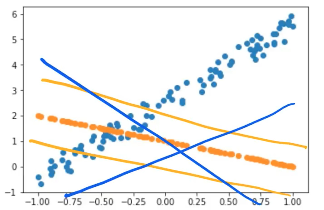
We want to find these parameters such that the line that they create minimizes the error between that line and the points.

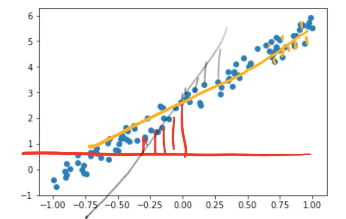
In other words, if the a₁ and a₂ we came up with resulted in red line. Then we’d look and we’d see how far away is that line from each point. That’s quite a long way.
So maybe there was some other a₁ and a₂ which resulted in the gray line. And they would say how far away is each of those points.
And then eventually we come up with the yellow line. In this case, each of those is actually very close.

So you can see how in each case we can say how far away is the line at each spot away from its point, and then we can take the average of all those. That’s called the loss. That is the value of our loss. So you need a mathematical function that can basically say how far away is this line from those points.

For this kind of problem which is called a regression problem (a problem where your dependent variable is continuous, so rather than being grizzlies or teddies, it’s some number between -1 and 6), the most common loss function is called mean squared error which pretty much everybody calls MSE. You may also see RMSE which is the root mean squared error. The mean squared error is a loss which is the difference between some predictions that you made which is like the value of the line and the actual number of ice cream sales. In the mathematics of this, people normally refer to the actual as y and the prediction, they normally call it

\hat{y}

(pronounced as y hat).

When writing something like mean squared error equation, there is no point writing “ice cream” and “temperature” because we want it to apply to anything. So we tend to use these mathematical placeholders.

So the value of the mean squared error is simply the difference between those two (y_hat - y) squared. Then we can take the mean because both y_hat and y are rank 1 tensors, so we subtract one vector from another vector, it does something called “element-wise arithmetic” in other words, it subtracts each one from each other, so we end up with a vector of differences. Then if we take the square of that, it squares everything in that vector. So then we can take the mean of that to find the average square of the differences between the actuals and the predictions.

def mse(y_hat, y) : 
    return ((y_hat-y)**2).mean()

If you’re more comfortable with mathematical notation then what we just wrote was

\frac{\sum(\hat{y}-y)^2}{n}

One of the things I’ll note here is, I don’t think ((y_hat-y)**2).mean() is more complicated or unwieldy than \frac{\sum(\hat{y}-y)^2}{n}

but the benefit of the code is you can experiment with it. Once you’ve defined it, you can use it, you can send things into it, get stuff out of it, and see how it works. So for Jeremy, most of the time, he prefers to explain things with code rather than with math. Because they are the same, just different notations. But one of the notations is executable. It’s something you can experiment with. And the other is abstract. That’s why I’m generally going to show the code.

So the good news is, if you’re a coder with not much of a math background, actually you do have a math background. Because the code is math. If you’ve got more of math background and less of a coding background, then actually a lot of the stuff that you learned from math is going to translate directly into the code and now you can start to experiment with your math.

mse is a loss function. This is something that tells us how good our line is. Now we have to come up with what is the line that fits through here. Remember, we are going to pretend we don’t know. So what you actually have to do is you have to guess. You actually have to come up with a guess what are the values of a₁ and a₂.

a = tensor(-1.,1)

Here is how you create that tensor and I wanted to write it this way because you’ll see this all the time. Written out fully, it would be tensor(-1.0, 1.0) . We can’t write it without the point because tensor(-1, 1)is an int, not a floating point. So that’s going to spit the dummy (Australian for “behave in a bad-tempered or petulant way”) if you try to do calculations with that in neural nets.

Jeremy is far too lazy to type .0 every time. Python knows perfectly well that if you added . next to any of these numbers, then the whole thing is now in floats. So that’s why you’ll often see it written this way, particularly by lazy people like us.

So a is a tensor. You can see it’s floating-point. You see, even PyTorch is lazy. They just put a dot. They don’t bother with a zero.

a = tensor(-1.,1)

a
tensor([-1.,  1.])

a.type()
'torch.FloatTensor'

But if you want to actually see exactly what it is, you can write .type() and you can see it’s a FloatTensor.

So now we can calculate our predictions with this random guess. x@a a matrix product of x and a. And we can now calculate the mean squared error of our predictions and their actuals, and that’s our loss. So for this regression, our loss is 8.9.

y_hat = x @ a 

mse(y_hat, y)
tensor(7.0485)

So we can now plot a scatter plot of x against y and we can plot the scatter plot of x against y_hat. And there they are.

plt.scatter(x[:,0],y)
plt.scatter(x[:,0],y_hat);

So that is not great, not surprising. It’s just a guess. So SGD or gradient descent more generally and anybody who’s done engineering or probably computer science at school would have done plenty of this like Newton’s method, etc at the university. If you didn’t, don’t worry. We’re going to learn it now.

It’s basically about taking this guess and trying to make it a little bit better. How do we make it a little better? Well, there are only two numbers and the two numbers are the intercept of the orange line and the gradient of the orange line. So what we are going to do with gradient descent is we’re going to simply say what if we changed those two numbers a little bit?

What if we made the intercept a little bit higher? (orange line)
What if we made the intercept a little bit lower? (orange line)
What if we made the gradient a little bit more positive? (blue line)
What if we made the gradient a little bit more negative? (blue line)

There are 4 possibilities and then we can calculate the loss for each of those 4 possibilities and see what works. Did lifting it up or down making it better? Did tilting it more positive or more negative make it better? And then all we do is we say, okay, whichever one of those made it better, that’s what we’re going to do. That’s it.

But here is the cool thing for those of you that remember calculus. You don’t actually have to move it up and down, and round about. You can actually calculate the derivative. The derivative is the thing that tells you would move it up or down to make it better or would rotating it this way or that way make it better. The good news is if you didn’t do calculus or you don’t remember calculus, I just told you everything you need to know about it. It tells you how changing one thing changes the function. That’s what the derivative is, kind of, not quite strictly speaking, but close enough, also called the gradient. The gradient or the derivative tells you how changing a₁ up or down would change our MSE, how changing a₂ up or down would change our MSE, and this does it more quickly than actually moving it up and down.

In school, unfortunately, they forced us to sit there and calculate these derivatives by hand. We have computers. Computers can do that for us. We are not going to calculate them by hand.

a = nn.Parameter(a); a
tensor([-1.,  1.], requires_grad=True)

Instead, we’re doing to call .grad() on our computer, that will calculate the gradient for us.

def update():
    y_hat = x@a
    loss = mse(y, y_hat)
    if t % 10 == 0: print(loss)
    loss.backward()
    with torch.no_grad():
        a.sub_(lr * a.grad)
        a.grad.zero_()

So here is what we’re going to do. We are going to create a loop. We’re going to loop through 100 times, and we’re going to call a function called update().

lr = 1e-1 for t in range(100): update()

tensor(7.0485, grad_fn=&lt;MeanBackward1&gt;) tensor(1.5014, grad_fn=&lt;MeanBackward1&gt;)
tensor(0.4738, grad_fn=&lt;MeanBackward1&gt;) tensor(0.1954, grad_fn=&lt;MeanBackward1&gt;) 
tensor(0.1185, grad_fn=&lt;MeanBackward1&gt;) tensor(0.0972, grad_fn=&lt;MeanBackward1&gt;) 
tensor(0.0913, grad_fn=&lt;MeanBackward1&gt;) tensor(0.0897, grad_fn=&lt;MeanBackward1&gt;) 
tensor(0.0892, grad_fn=&lt;MeanBackward1&gt;) tensor(0.0891, grad_fn=&lt;MeanBackward1&gt;)

This function is going to:

Calculate y_hat (i.e. our prediction)
Calculate loss (i.e. our mean squared error)
From time to time, it will print that out so we can see how we’re going
Calculate the gradient. In PyTorch, calculating the gradient is done by using a method called backward(). Mean squared error was just a simple standard mathematical function. PyTorch for us keeps track of how it was calculated and lets us calculate the derivative. So if you do a mathematical operation on a tensor in PyTorch, you can call backward() to calculate the derivative and the derivative gets stuck inside an attribute called .grad.
Take my coefficients and I’m going to subtract from them my gradient (a.sub_()). There is an underscore there because that’s going to do it in-place. It’s going to actually update those coefficients a to subtract the gradients from them. Why do we subtract? Because the gradient tells us if I move the whole thing downwards, the loss goes up. If I move the whole thing upwards, the loss goes down. So I want to do the opposite of the thing that makes it go up. We want our loss to be small. That’s why we subtract.
lr is our learning rate. All it is is the thing that we multiply by the gradient. Why is there any lr at all? Let me show you why.

What is the need for learning rate [1:41:32]

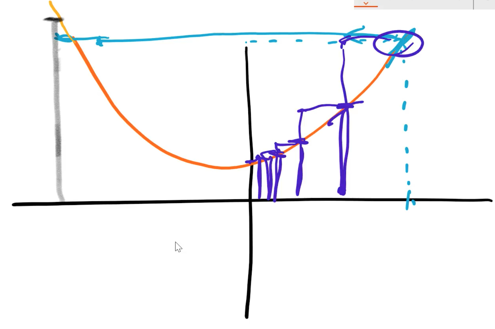
Let’s take a really simple example, a quadratic. And let’s say your algorithm’s job was to find where that quadratic was at its lowest point. How could it do this? Just like what we’re doing now, the starting point would be just to pick some x value at random. Then find out what the value of y is. That’s the starting point. Then it can calculate the gradient and the gradient is simply the slope, but it tells you moving in which direction makes you go down. So the gradient tells you, you have to go this way.

If the gradient was really big, you might jump left a very long way, so you might jump all the way over to here. If you jumped over there, then that’s actually not going to be very helpful because it’s worse. We jumped too far so we don’t want to jump too far.
Maybe we should just jump a little bit. That is actually a little bit closer. So then we’ll just do another little jump. See what the gradient is and do another little jump, and repeat.
In other words, we find our gradient to tell us what direction to go and if we have to go a long way or not too far. But then we multiply it by some number less than 1 so we don’t jump too far.

Hopefully, at this point, this might be reminding you of something which is what happened when our learning rate was too high.

learn = create_cnn(data, models.resnet34, metrics=error_rate)

learn.fit_one_cycle(1, max_lr=0.5)

Total time: 00:13
epoch  train_loss  valid_loss  error_rate       
1      12.220007   1144188288.000000  0.765957    (00:13)

Do you see why that happened now? Our learning rate was too high meant that we jumped all the way past the right answer further than we started with, and it got worse, and worse, and worse. So that’s what a learning rate too high does.

On the other hand, if our learning rate is too low, then you just take tiny little steps and so eventually you’re going to get there, but you are doing lots and lots of calculations along the way. So you really want to find something where it’s either big enough steps like stairs or a little bit of back and forth. You want something that gets in there quickly but not so quickly it jumps out and diverges, not so slowly that it takes lots of steps. That’s why we need a good learning rate and that’s all it does.

So if you look inside the source code of any deep learning library, you’ll find this:

a.sub_(lr * a.grad)

You will find something that says “coefficients ﹣ learning rate times gradient”. And we will learn about some easy but important optimization we can do to make this go faster.

That’s about it. There’s a couple of other little minor issues that we don’t need to talk about now: one involving zeroing out the gradient and other involving making sure that you turn gradient calculation off when you do the SGD update. If you are interested, we can discuss them on the forum or you can do our introduction to machine learning course which covers all the mechanics of this in more detail.

Training loop [1:45:45]

If we run update() 100 times printing out the loss from time to time, you can see it starts at 8.9, and it goes down.

lr = 1e-1

for t in range(100): update()

tensor(8.8945, grad_fn=<MeanBackward1>)
tensor(1.6115, grad_fn=<MeanBackward1>)
tensor(0.5759, grad_fn=<MeanBackward1>)
tensor(0.2435, grad_fn=<MeanBackward1>)
tensor(0.1356, grad_fn=<MeanBackward1>)
tensor(0.1006, grad_fn=<MeanBackward1>)
tensor(0.0892, grad_fn=<MeanBackward1>)
tensor(0.0855, grad_fn=<MeanBackward1>)
tensor(0.0843, grad_fn=<MeanBackward1>)
tensor(0.0839, grad_fn=<MeanBackward1>)

So you can then print out scatterplots and there it is.

plt.scatter(x[:,0],y)
plt.scatter(x[:,0],x@a);

Animation of SGD update [1:46:21]

Let’s now take a look at this as an animation. This is one of the nice things that you can do with matplotlib. You can take any plot and turn it into an animation. So you can now actually see it updating each step.

from matplotlib import animation, rc 
rc('animation', html='html5')

You may need to uncomment the following to install the necessary plugin the first time you run this: (after you run following commands, make sure to restart the kernel for this notebook) If you are running in colab, the installs are not needed; just change the cell above to be … html=‘jshtml’ instead of … html=‘html5’

#! sudo add-apt-repository -y ppa:mc3man/trusty-media 
#! sudo apt-get update -y 
#! sudo apt-get install -y ffmpeg 
#! sudo apt-get install -y frei0r-plugins

Let’s see what we did here. We simply said, as before, create a scatter plot, but then rather than having a loop, we used matplotlib’s FuncAnimation to call 100 times this animate function. And this function just calls that update we created earlier and then update the y data in our line. Repeat that 100 times, waiting 20 milliseconds after each one.

a = nn.Parameter(tensor(-1.,1))

fig = plt.figure()
plt.scatter(x[:,0], y, c='orange')
line, = plt.plot(x[:,0], x@a)
plt.close()

def animate(i):
    update()
    line.set_ydata(x@a)
    return line,

animation.FuncAnimation(fig, animate, np.arange(0, 100), interval=20)

You might think visualizing your algorithms with animations is something amazing and complex thing to do, but actually, now you know it’s 11 lines of code. So I think it’s pretty damn cool.

That is SGD visualized and we can’t visualize as conveniently what updating 50 million parameters in a ResNet 34 looks like but basically doing the same thing. So studying these simple version is actually a great way to get an intuition. So you should try running this notebook with a really big learning rate, with a really small learning rate, and see what this animation looks like, and try to get a feel for it. Maybe you can even try a 3D plot. I haven’t tried that yet, but I’m sure it would work fine.

Mini-batches [1:48:05]

The only difference between stochastic gradient descent and this is something called mini-batches. You’ll see, what we did here was we calculated the value of the loss on the whole dataset on every iteration. But if your dataset is 1.5 million images in ImageNet, that’s going to be really slow. Just to do a single update of your parameters, you’ve got to calculate the loss on 1.5 million images. You wouldn’t want to do that. So what we do is we grab 64 images or so at a time at random, and we calculate the loss on those 64 images, and we update our weights. Then we have another 64 random images, and we update our weights. In other words, the loop basically looks exactly the same but add some random indexes on our x and y to do a mini-batch at a time, and that would be the basic difference.

def update():
    y_hat = x@a
    loss = mse(y, y_hat)
    if t % 10 == 0: print(loss)
    loss.backward()
    with torch.no_grad():
        a.sub_(lr * a.grad)
        a.grad.zero_()

Once you add those grab a random few points each time, those random few points are called your mini-batch, and that approach is called SGD for Stochastic Gradient Descent.

Vocabulary [1:49:42]

There’s quite a bit of vocab we’ve just covered, so let’s remind ourselves.

Learning rate: A thing we multiply our gradient by to decide how much to update the weights by.
Epoch: One complete run through all of our data points (e.g. all of our images). So for non-stochastic gradient descent we just did, every single loop, we did the entire dataset. But if you’ve got a dataset with a thousand images and our mini-batch size is 100, then it would take you 10 iterations to see every image once. So that would be one epoch. Epochs are important because if you do lots of epochs, then you are looking at your images lots of times, so every time you see an image, there’s a bigger chance of overfitting. So we generally don’t want to do too many epochs.
Mini-batch: A random bunch of points that you use to update your weights.
SGD: Gradient descent using mini-batches.
Model / Architecture: They kind of mean the same thing. In this case, our architecture is

the architecture is the mathematical function that you’re fitting the parameters to. And we’re going to learn later today or next week what the mathematical function of things like ResNet34 actually is. But it’s basically pretty much what you’ve just seen. It’s a bunch of matrix products.

Parameters / Coefficients / Weights : Numbers that you are updating.
Loss function: The thing that’s telling you how far away or how close you are to the correct answer. For classification problems, we use cross entropy loss, also known as negative log-likelihood loss. This penalizes incorrect confident predictions, and correct unconfident predictions.

1:51:45

These models/predictors/teddy bear classifiers are functions that take pixel values and return probabilities. They start with some functional form like and they fit the parameter a using SGD to try and do the best to calculate your predictions. So far, we’ve learned how to do regression which is a single number. Next, we’ll learn how to do the same thing for classification where we have multiple numbers, but basically the same.

In the process, we had to do some math. We had to do some linear algebra and calculus and a lot of people get a bit scared at that point and tell us “I am not a math person”. If that’s you, that’s totally okay. But you are wrong. You are a math person. In fact, it turns out that in the actual academic research around this, there are not “math people” and “non-math people”. It turns out to be entirely a result of culture and expectations. So you should check out Rachel’s talk:

There is no such thing as “not a math person”

She will introduce you to some of that academic research. If you think of yourself as not a math person, you should watch this so that you learn that you’re wrong that your thoughts are actually there because somebody has told you-you’re not a math person. But there’s actually no academic research to suggest that there is such a thing. In fact, there are some cultures like Romania and China where the “not a math person” concept never even appeared. It’s almost unheard of in some cultures for somebody to say I’m not a math person because that just never entered that cultural identity.

So don’t freak out if words like derivative, gradient, and matrix product are things that you’re kind of scared of. It’s something you can learn. Something you’ll be okay with.

Underfitting and Overfitting [1:54:45]

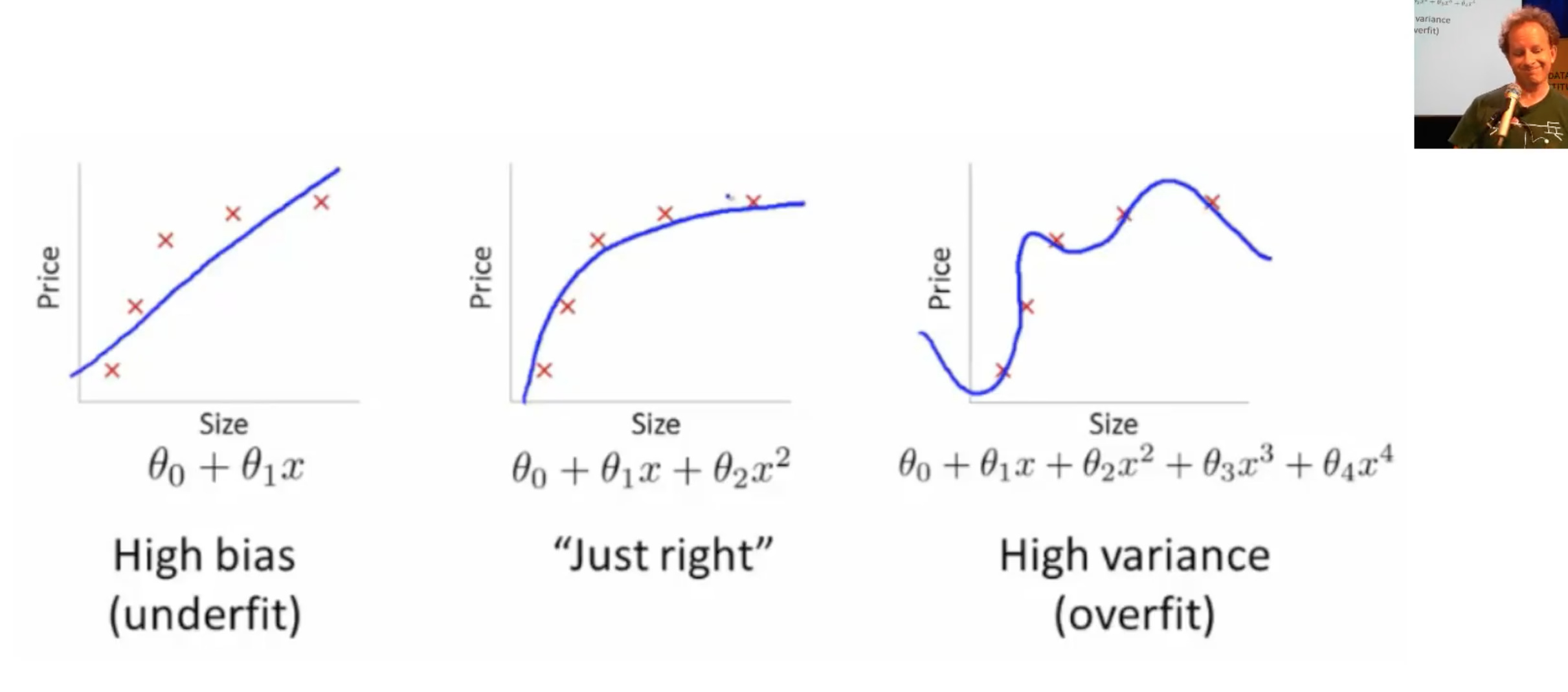
The last thing I want to close with is the idea of underfitting and overfitting. We just fit a line to our data. But imagine that our data wasn’t actually line-shaped.

1. Underfitting -

So if we try to fit which was something like constant + constant times X (i.e. a line) to it, it’s never going to fit very well. No matter how much we change these two coefficients, it’s never going to get really close.

2. Overfitting -

On the other hand, we could fit some much bigger equation, so in this case, it’s a higher degree polynomial with lots of wiggly bits. But if we did that, it’s very unlikely we go and look at some other place to find out the temperature and how much ice cream they are selling and we will get a good result. Because the wiggles are far too wiggly. So this is called overfitting.

3. Just right -

We are looking for some mathematical function that fits just right to stay with a teddy bear analogies. You might think if you have a statistics background, the way to make things it just right is to have exactly the same number of parameters (i.e. to use a mathematical function that doesn’t have too many parameters in it). It turns out that’s actually completely not the right way to think about it.

Regularization and Validation Set [1:56:07]

There are other ways to make sure that we don’t overfit. In general, this is called regularization. Regularization or all the techniques to make sure when we train our model that it’s going to work not only well on the data it’s seen but on the data it hasn’t seen yet. The most important thing to know when you’ve trained a model is actually how well does it work on data that it hasn’t been trained with. As we’re going to learn a lot about next week, that’s why we have this thing called a validation set.

What happens with the validation set is that we do our mini-batch SGD training loop with one set of data with one set of teddy bears, grizzlies, black bears. Then when we’re done, we check the loss function and the accuracy to see how good is it on a bunch of images which were not included in the training. So if we do that, then if we have something which is too wiggly, it will tell us. “Oh, your loss function and your error are really bad because on the bears that it hasn’t been trained with, the wiggly bits are in the wrong spot.” Or else if it was underfitting, it would also tell us that your validation set is really bad.

Even for people that don’t go through this course and don’t learn about the details of deep learning, if you’ve got managers or colleagues at work who are wanting to learn about AI, the only thing that you really need to be teaching them is about the idea of a validation set. Because that’s the thing they can then use to figure out if somebody’s telling them snake oil or not. They hold back some data and they get told “oh, here’s a model that we’re going to roll out” and then you say “okay, fine. I’m just going to check it on this held out data to see whether it generalizes.” There’s a lot of details to get right when you design your validation set. We will talk about them briefly next week, but a more full version would be in Rachel’s piece on the fast.ai blog called How (and why) to create a good validation set. And this is also one of the things we go into in a lot of detail in the intro to machine learning course. So we’re going to try and give you enough to get by for this course, but it is certainly something that’s worth deeper study as well.

Thanks, everybody! Jeremy hopes we have a great time building our web applications. See you next week.

devforfu · October 31, 2018, 9:33am

As a small note, x@a works since Python >= 3.5, for anyone who still should use earlier versions.

PoonamV · October 31, 2018, 9:56am

@jeremy can you turn this post into wiki.

PoonamV · October 31, 2018, 9:56am

Thanks, added in notes.

cedric · October 31, 2018, 10:41am

Hi Poonam, thank you again for starting this. While we wait for Jeremy to turn this post into wiki, could you please add the common header section to your notes and link back to lesson 1 notes?

I have linked to this notes from lesson 1 notes and from the “lesson 2 official resources and updates”. Thanks.

PoonamV · October 31, 2018, 11:13am

Thanks Cedric. will surely do that.

balnazzar · October 31, 2018, 12:18pm

Great notes, thank you fr sharing!

boy1729 · October 31, 2018, 1:09pm

Pasting the link here so that if thread is converted into wiki, this is not lost:

jeremy · October 31, 2018, 4:15pm

Done.

bsalita · October 31, 2018, 6:23pm

If you find that the javascript code, which collects urls into a download file, isn’t producing the file or the file is zero length, you may have an ad blocker or popup blocker that’s interfering. Turn off the blocker, refresh the page and try the javascript again. In my case, uBlockOrigin was causing a problem.

Also the javascript doesn’t seem to work on Windows in Microsoft Edge, Firefox, or a private/incognito window. Can anyone verify? It only works in Chrome.

Lankinen · November 1, 2018, 8:16am

I got my personal notes ready and as soon as I have time I will copy some parts from there to here. If someone is interested to read my notes and finds something interesting, with my permission you can just copy past it to these notes. And again if there is too much information to be shared publicly reply this message and I will delete that post. Thanks again to Jeremy this amazing lesson.

cedric · November 6, 2018, 12:45pm

Detailed lesson 2 notes by Hiromi.

abhinow · November 23, 2018, 2:31pm

While picking a learning rate, when do we pick 3e-5 vs 1e-5 ? There was a part of the video in lesson 2 where Jeremy saw the image and put 3e-5 and I wasn’t sure when 1e-5 would be used against 3e-5

AshwaniTiwari · April 8, 2019, 7:57am

After download the url on the local , I have to uplaod that url on the kaggle . The directory created by the python code is “data/beers/…” , then how to upload the file from local to this directory location , because from the “Add Dataset” option on the kaggel , dosent show me this location. Please help me .

homofortis · June 1, 2019, 6:52am

Here is the javascript to download the links In case you are using DuckDuckGo instead of Google to search for images:
urls = Array.from(document.querySelectorAll('img.tile--img__img.js-lazyload')).map(el=>decodeURIComponent(el.src.split('=')[1])); window.open('data:text/csv;charset=utf-8,' + escape(urls.join('\n')));

matejthetree · June 4, 2019, 12:21am

I created SGD for square functions. I hope this is the right place to post it
https://www.kaggle.com/matejthetree/sgd-2?scriptVersionId=15140809
I am bad with plot, so I dont know why it pops two images at the end

lymenlee · September 10, 2019, 10:05pm

I manged to download some images of different Chinese Calligraphy artworks. Plan is to build a Chinese calligraphy style classifier. I did all the work on a Kaggle Kernel and uploaded images as private dataset to be used by the kernel. My question may be quite dumb, but what kind of license should I use for the dataset? Or should I upload to Kaggle at all without breaking some license? I want to share the notebook on Kaggle once I finished, but if license won’t clear, I don’t think I can do that. Anyone here could shed some lights on this topic? Much appreciated!

gbubs · September 17, 2019, 5:57pm

Does anyone know why my epochs always start from zero instead of one (when I run learn.fit_one_cycle)?
Also why Jeremy used max_lr slice (3e-5, 3e-4) instead of (1e-5, 1e-4) (after running learn.recorder.plot())?

amit_js · September 29, 2019, 10:04am

Can Some one please turn this into a set of equations, Especially the

loss.backward()
 with torch.no_grad():
        a.sub_(lr * a.grad)
        a.grad.zero_()

I’m having a hard time understanding it.

farid · September 30, 2019, 2:24pm

a : is the weight tensor (that also stores its gradient in a.grad ) that our model will determine during the training of our model (y = x @ a)
a.grad is an attribute of the a tensor where the gradient of a is stored

a.grad is calculated after each call of the loss.backward() function
Then a is update like this
a = a - lr * a.grad
which can be written like this
a -= lr * a.grad
And in pytorch, it is written like this
a.sub_(lr*a.grad)
it’s called in-place sub() because it directly updates the a tensor in-place

(by the way, if you see a function that ends with _ like sub_(), it means it’s an in-place version of its correspondent function (like add and add_) : It’s a convention)

Once we finish updating the a tensor, we have to reset a.grad to zero ( a.grad.zero_() ) before calling the next loss.backward() function.

As for the with torch.no_grad(): , we use it to ask pytorch to stop updating (tracking) a.grad (it’s already calculated after the loos.backward() call) while we are updating the a tensor