<<< Notes: Lesson 5 | Notes: Lesson 7 (TBA) >>>
Thanks, Jeremy for another great lecture.
Hi everybody, welcome to lesson 6.
Important posts to watch:
Software Update
![]() Always remember to do an update on fast.ai library and course repo.
Always remember to do an update on fast.ai library and course repo.
conda install -c fastai fastai for the library update
git pull for the course repo update.
Lesson 6 Notebooks:
Introduction
We’re going to do a deep dive into computer vision convolutional neural networks what is a convolution and we’re also going to learn the final regularization tricks after the last lesson learning about weight decay and/or l2 regularization.
Jeremy is really excited about and he has had a small hand and helping to create.
For those of you that saw his talk on ted.com, you might have noticed this really interesting demo that we did about four years ago showing a way to quickly build models with unlabeled data.
Jeremy Howard - The wonderful and terrifying implications of computers that can learn
Quick demo about platform.ai

It’s been for years but we’re finally at a point where we’re ready to put this out in the world and let people use it and the first people we’re going to let use it are you folks so the company is called platform.ai.
The reason Jeremy is mentioning it here is that it’s going to let you create models on different types of data sets to what you can do now that is to say data sets that you don’t have labels for yet. the platform.ai actually going to help you label them. This is the first time this has been shown before so Jeremy is pretty thrilled about it.
If you’d go to platform.ai and choose to get started you’ll be able to create a new project and if you create a new project you can either upload your own images. Uploading it at 500 or so works pretty well.
You can upload a few thousand but you know to start upload 500 or so they all have to be in a single folder and so we’re assuming that you’ve got a whole bunch of images that you haven’t got any labels for.
Or you can start with one of the existing collections if you want to play around.
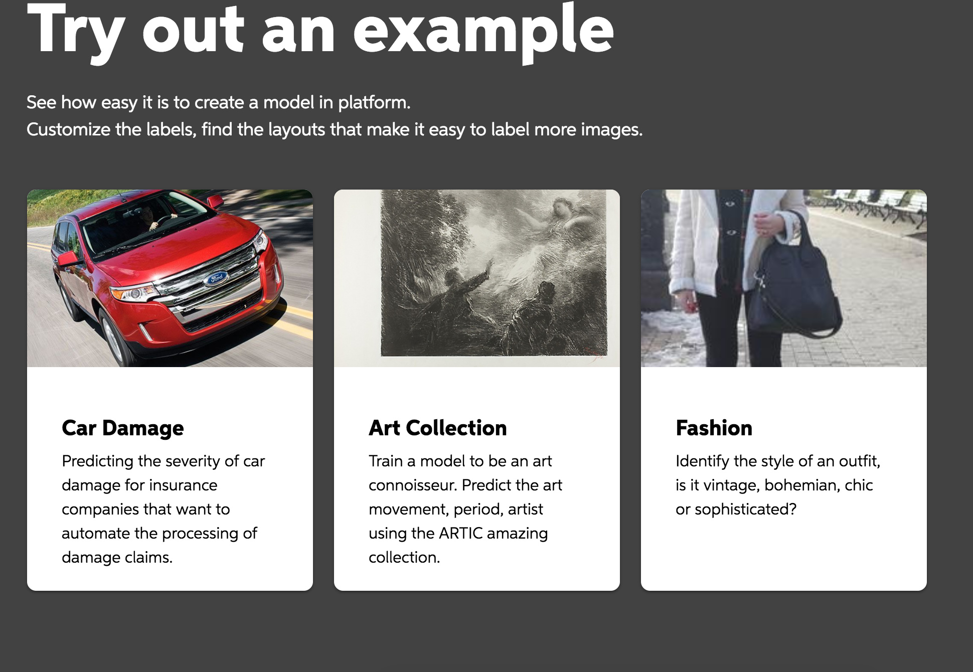
Jeremy has started with the cars collection kind of going back to what we did 4 years ago and so this is what happens when you first go into platform.ai and look at the collection of images you’ve uploaded a random sample of them will appear on the screen. As you’ll recognize probably they are projected from a deep learning space into a 2d space using a pre-trained model and for this initial version, it’s an Imagenet model we’re using. As things move along we’ll be adding more and more pre-trained models and what Jeremy wants to add labels to this data set representing which angle a photo of the car was taken from. Which is something that actually images that’s going to be really bad at isn’t it? Because Imagenet has learned to recognize the difference between cars versus bicycles and Imagenet knows that the angle you take a photo on actually doesn’t matter. So we want to try and create labels using the kind of thing that actually image net specifically learned to ignore. The projection that you see we can click these layer buttons at the top to switch to user projection using a different layer of the neural net.
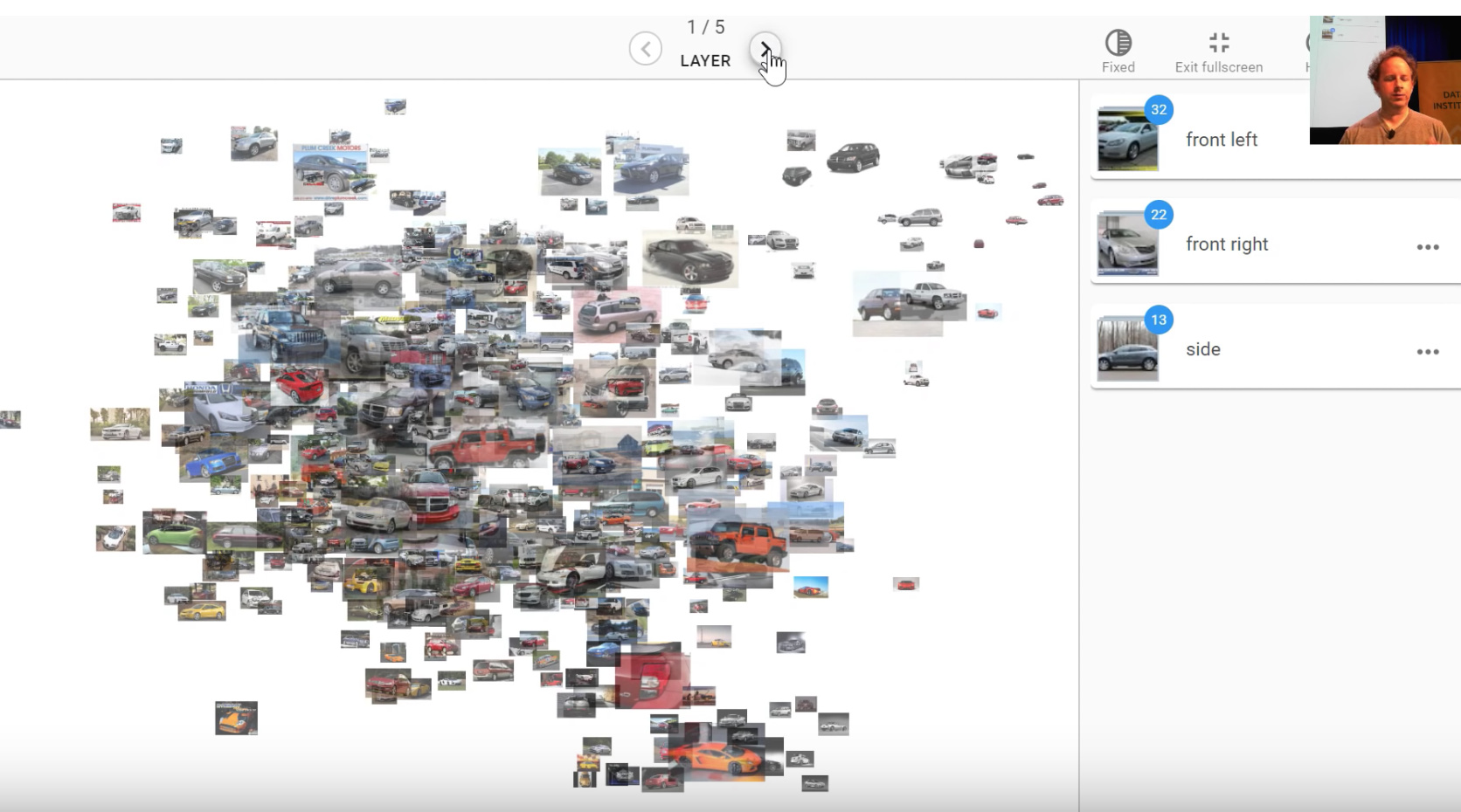
Here’s the last layer which is going to be a total waste of time for us because it’s really going to be projecting things based on what kind of thing it thinks it is and the first layer is probably going to be the same for us as well because there’s very little interesting semantic content there.
But if we go into the middle in layer 3 we may well be able to find some differences there so then what you can do is you can click on the projection button here.
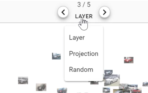
you can actually just press up and down rather than just pressing the arrows at the top to switch between projections or left and right. You can basically look around until you notice that there’s a projection which is kind of separated out things you’re interested in and so this one actually Jeremy notices that it’s got a whole bunch of cars that are kind of front right. If we zoom in a little bit we can double check because like yeah that looks pretty good they’re all kind of front right so we can click on here to go to selection mode and we can cut a grab a few and then you should check.
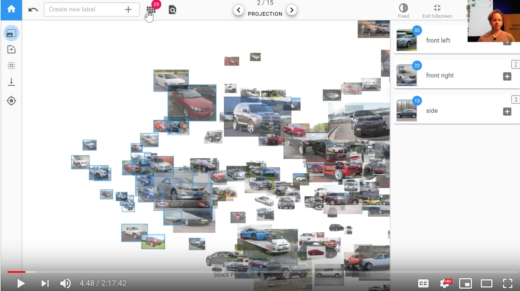

What we’re doing here is we’re trying to take advantage of the combination of the human plus machine the machine is pretty good at quickly doing calculations but as a human, we’re pretty good at looking at a lot of things at once and seeing the odd one out. In this case, we’re looking for cars that aren’t front right and so by laying the one on in front of us we can do that really quickly it’s like okay definitely that one so just click on the ones that you don’t want all right it’s all good so then you can just go back and so then what you can do is you can either put them into a new category but I can create a new label or you can click on one of the existing ones so before Jeremy came he just created a few so here’s front right so he just clicks on it here there we go .
Rossman Store Sales Kaggle competition
From last week’s discussion of regularization specifically in the context of the tabular learner. This was the init method in the tabular learner
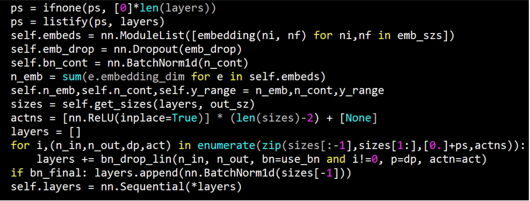
Our goal was to understand everything here and we’re not quite there yet. Last week we were looking at the adult data set which is a really simple data set that’s just for toy purposes. So this week let’s look at a data set that’s much more interesting a Kaggle competition dataset. We know kind of what the best in the world and you know Kaggle competition results tend to be much harder to beat than academic state-of-the-art results tend to be because of a lot more people work on Kaggle competitions than most academic data sets. It’s a really good challenge to try and do well on a Kaggle competition dataset. The Rossmann data set is if they’ve got three thousand drugs in Europe and you’re trying to predict how many products they’re going to sell in the next couple of weeks.
Interesting stuff
-
The test set for this is from a time period that is more recent than the training set. This is really common if you want to predict things there’s no point predicting things that are in the middle of your training set you want to predict things in the future.
-
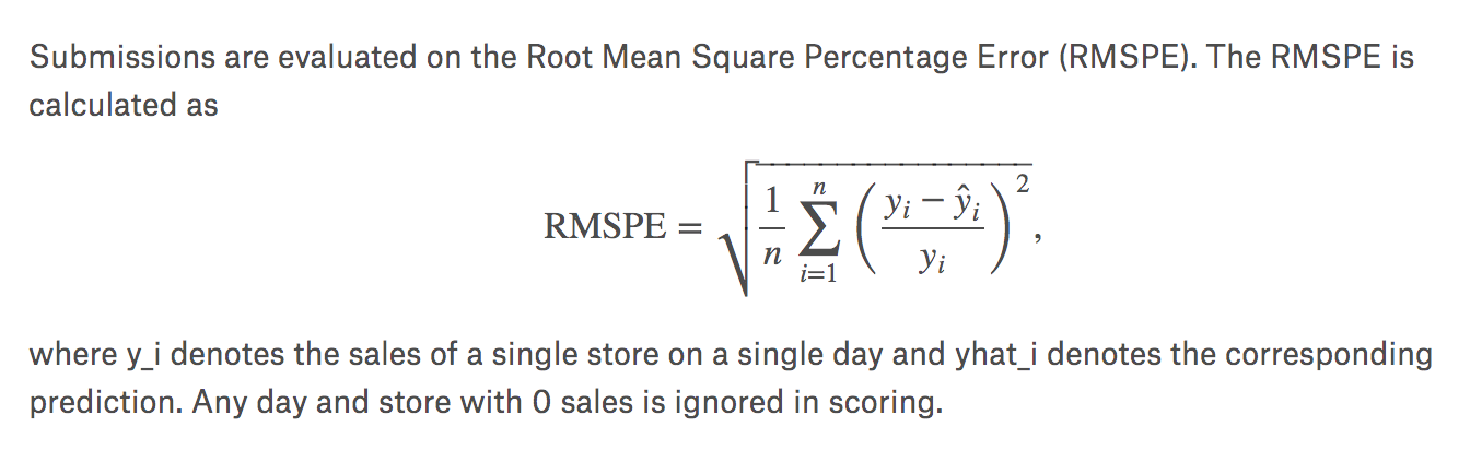
The evaluation metric they provided is the root mean squared percent error so this is just a normal root mean squared error except we go actual minus prediction divided by actual.
It’s the percent error that we’re taking the root mean square of.
-
It’s always interesting to look at the leaderboard. The leaderboard the winner was 0.1. The paper that we’ve roughly replicated was point 105 106 and 10th place out of 3,000 was 0.11 ish bit less.
Additional data
The data that was provided by Kaggle has a small number of files. But they also let competitors provide additional external data as long as they shared it with all the competitors. In practice, the data the set we’re going to use contains 6 or 7 tables. The way that you join tables and stuff isn’t really part of a deep learning course so Jeremy is going to skip over it and instead refers you to Introduction to machine learning for coders which will take you step-by-step through the data preparation. For now, it’s readily available in course repo
You’ll see the whole process there.
You’ll need to run through rossman_data_clean.iynb notebook to create these pickle files that we read here.
from fastai.tabular import *
path = Path('data/rossmann/')
train_df = pd.read_pickle(path/'train_clean')
Jeremy just wants to mention one particularly interesting part of the rossmann_data_clean.ipynb notebook which is you’ll see there’s something that says add_date() part.
train_df.head().T

Jeremy has been mentioning about time series and pretty much everybody assumed he’s going to do some kind of recurrent neural network but he’s not. Interestingly the kind of the main academic group that studies time series is econometrics. They tend to study one very specific kind of time series which is where the only data you have is a sequence of time points of one thing that’s the only thing you have is one sequence.
In real life that’s have is one sequence in real life that’s almost never the case. Normally you know if we would have some information about the store or the people that it represents we’d have metadata. We’d have sequences of other things measured at similar time periods or different time periods.
Most of the time Jeremy finds in practice the state-of-the-art results when it comes to competitions on kind of more real-world data sets don’t tend to its recurrent neural networks. But instead they tend to take it’s a timepiece which in this case it was a date we were given in the data and they add a whole bunch of metadata.
add_datepart(train, "Date", drop=False)
add_datepart(test, "Date", drop=False)
In our case, for example, we’ve added the day of the week. We were given a date right we’ve had a day of week year, month, week of the year, the day of the month, the day of the week, the day of the year and then a bunch of boolean is it the month start or end?, quarter start or end?, year start or end? and elapsed time since 1970 so forth. If you run this one function add_date_part() and pass it date it’ll add all of these columns to your data set for you.
What that means is that let’s take a very reasonable example, purchasing behavior probably changes on payday. Payday might be the fifteenth of the month so if you have this day of the month here. Then it’ll be able to recognize every time something is a fifteen there and associated it with a higher in this case embedding matrix value. but so this way it basically you know we can’t expect a neural net to do all of our feature engineerings for us. We can expect the neural network to kind of find nonlinearities and interactions and stuff like that. But for something like taking a date like this and figuring out that the fifteenth of the month is something when interesting things happen it’s much better if we can provide that information for the neural network manually. so this is a really useful function to use and once you’ve done this you can treat many kinds of time-series problems as regular tabular problems. Jeremy says many kinds, not all. If there’s very complex kind of state involved in a time series such as you know equity trading or something like that this probably won’t be the case. Or this won’t be the only thing you need. But, in this case, it’ll get us a really good result.
In practice, most of the time Jeremy finds this works well.
Tabular data is normally in pandas so we just stored them as standard Python pickle files we can read them in. We can take a look at the first five records using df.head() and so the key thing here is that we’re trying to on a particular date for a particular store ID we want to predict the number of sales. The number of sales is the dependent variable
Processors
You’ve already learned about transforms. Transforms are bits of code that run every time something is grabbed from a data set. It’s really good for data augmentation that we’ll learn about today which is that it’s going to get a different random value every time it’s sampled. Pre-processors are like transforms but they’re a little bit different which is that they run once before you do any training. Really importantly they run once on the training set and then any kind of stage or metadata that’s created is then shared with the validation and test set. Jeremy gives an example when we’ve been doing image recognition and we’ve had a set of classes like all the different pet breeds and they’ve been turned into numbers. The thing that’s actually doing that for us is a preprocessor that’s being created in the background. So that makes sure that the classes for the training set are the same as the classes for the validation and the classes of the test set. We’re going to do something very similar here.
For example, if we create a small subset of data for playing with. This is a really good idea when you start with a new data set. Jeremy has just grabbed 2,000 IDs at random. He’s just going to grab a little training set and a little test set. Half and half of those 2,000 IDs. He’s going to grab five columns. Then we can just play around with this.
Experimenting with a sample

idx = np.random.permutation(range(n))[:2000]
idx.sort()
small_train_df = train_df.iloc[idx[:1000]]
small_test_df = train_df.iloc[idx[1000:]]
small_cont_vars = ['CompetitionDistance', 'Mean_Humidity']
small_cat_vars =  ['Store', 'DayOfWeek', 'PromoInterval']
small_train_df = small_train_df[small_cat_vars + small_cont_vars + ['Sales']]
small_test_df = small_test_df[small_cat_vars + small_cont_vars + ['Sales']]

small_train_df.head()
| Store | DayOfWeek | PromoInterval | CompetitionDistance | Mean_Humidity | Sales |
|---|---|---|---|---|---|
| 280 | 281 | 5 | NaN | 6970.0 | 61 |
| 584 | 586 | 5 | NaN | 250.0 | 61 |
| 588 | 590 | 5 | Jan,Apr,Jul,Oct | 4520.0 | 51 |
| 847 | 849 | 5 | NaN | 5000.0 | 67 |
| 896 | 899 | 5 | Jan,Apr,Jul,Oct | 2590.0 | 55 |
Here’s the first few of those from the training set.
3 Types of Preprocessors in fastai
Categorify
You can see one of the column is called promo interval. It has these strings(Jan, Apr, Jul, Oct) and sometimes it’s missing in pandas i.e, NAN. The first preprocessor Jeremy will show us is the Categorify and Categorify does basically the same thing that classes thing for image recognition does for a dependent variable. It’s going to take these strings it’s going to find all of the possible unique values of it and it’s going to create a list of them and then it’s going to turn the strings into numbers. If we call it on the training set that’ll create categories there and then we call it on our test set passing in test=true that makes sure it’s going to use the same categories that we had before. Now when we say small_train_df.head() it looks exactly the same.
small_test_df.head()
| Store | DayOfWeek | PromoInterval | CompetitionDistance | Mean_Humidity | Sales | |
|---|---|---|---|---|---|---|
| 428412 | NaN | 2 | NaN | 840.0 | 89 | 8343 |
| 428541 | 1050.0 | 2 | Mar,Jun,Sept,Dec | 13170.0 | 78 | 4945 |
| 428813 | NaN | 1 | Jan,Apr,Jul,Oct | 11680.0 | 85 | 4946 |
| 430157 | 414.0 | 6 | Jan,Apr,Jul,Oct | 6210.0 | 88 | 6952 |
| 431137 | 285.0 | 5 | NaN | 2410.0 | 57 | 5377 |
That’s because pandas have turned this into a categorical variable which internally is storing numbers but externally is showing us the strings. But we can look inside promo interval to look at the cat categories.
small_train_df.PromoInterval.cat.categories

Index(['Feb,May,Aug,Nov', 'Jan,Apr,Jul,Oct', 'Mar,Jun,Sept,Dec'], dtype='object')
This is all standard pandas here to show me a list of all of them what we would call classes in fastai or would be called just categories in pandas. If I look at the cat codes
small_train_df['PromoInterval'].cat.codes[:5]
280      -1
584      -1
588       1
847      -1
896       1
You can see this list here is the numbers that are actually stored -1, -1, 1, -1, 1.
So what are these -1’s? The -1’s represent NAN. They are missing so pandas use the special code -1 to mean missing value. Now as you know these are going to end up in an embedding matrix and we can’t look up item -1 in an embedding matrix so internally in fastai, we add 1 to all of these.
FillMissing
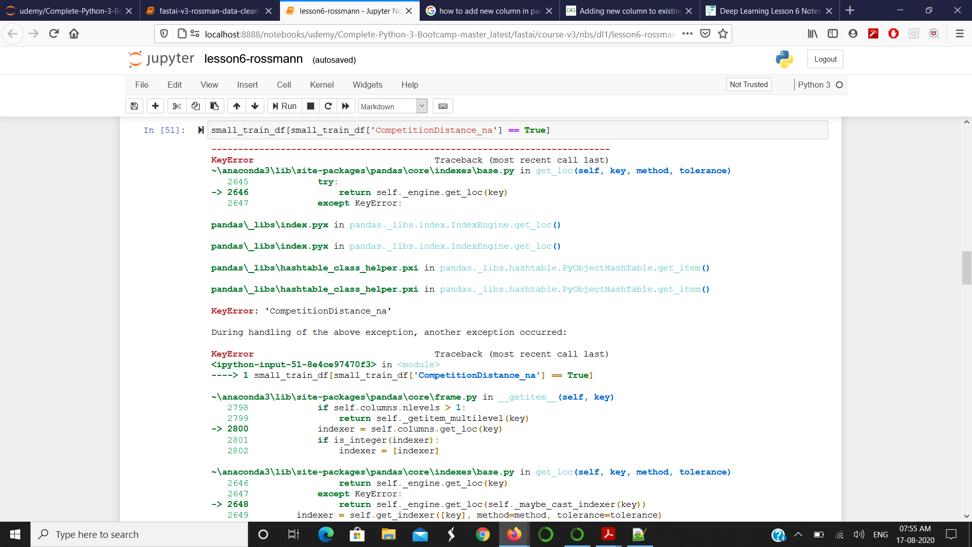
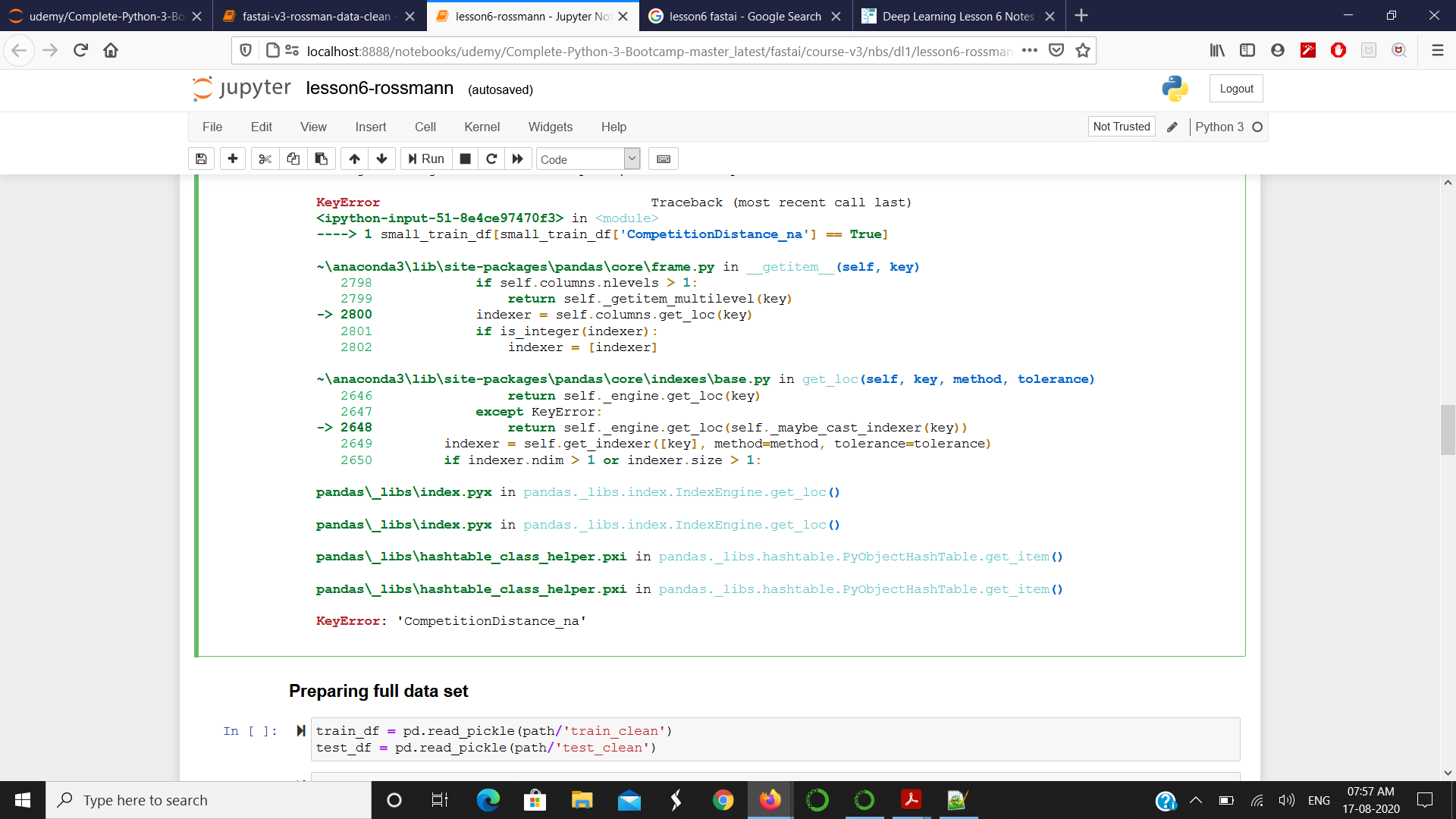
Another useful preprocessor is FillMissing and so again you can call it on the data frame you can call on the test passing in test = true.
fill_missing = FillMissing(small_cat_vars, small_cont_vars) fill_missing(small_train_df) fill_missing(small_test_df, test=True)

small_train_df[small_train_df['CompetitionDistance_na'] == True]
| Store | DayOfWeek | PromoInterval | CompetitionDistance | Mean_Humidity | Sales | CompetitionDistance_na | |
|---|---|---|---|---|---|---|---|
| 78375 | 622 | 5 | NaN | 2380.0 | 71 | 5390 | True |
| 161185 | 622 | 6 | NaN | 2380.0 | 91 | 2659 | True |
| 363369 | 879 | 4 | Feb,May,Aug,Nov | 2380.0 | 73 | 4788 | True |
This will create for everything that’s missing anything that has a missing value it’ll create an additional column with the column name _na so CompetitionDistance_na and it will set it to ‘True’ for any time that was missing. Then what we do is we replace competition distance with the median for those.