Wiki: Lesson 5

<<< Wiki: Lesson 4Wiki: Lesson 6 >>>

Lesson resources

Links to more info

Other datasets available

Video timeline

  • 00:00:01 Review of students articles and works

  • 00:07:45 Starting the 2nd half of the course: what’s next ?
    MovieLens dataset: build an effective collaborative filtering model from scratch

  • 00:12:15 Why a matrix factorization and not a neural net ?
    Using Excel solver for Gradient Descent ‘GRG Nonlinear’

  • 00:23:15 What are the negative values for ‘movieid’ & ‘userid’, and more student questions

  • 00:26:00 Collaborative filtering notebook, ‘n_factors=’, ‘CollabFilterDataset.from_csv’

  • 00:34:05 Dot Product example in PyTorch, module ‘DotProduct()’

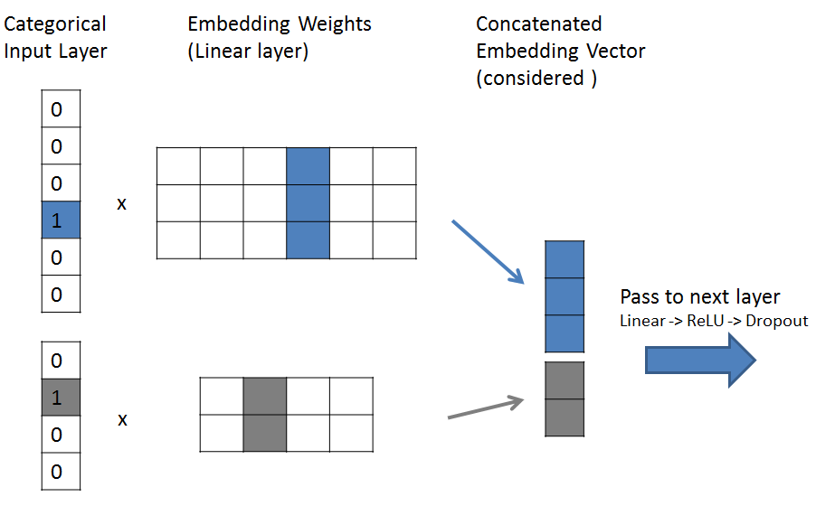
  • 00:41:45 Class ‘EmbeddingDot()’

  • 00:47:05 Kaiming He Initialization (via DeepGrid),
    sticking an underscore ‘_’ in PyTorch, ‘ColumnarModelData.from_data_frame()’, ‘optim.SGD()’

  • Pause

  • 00:58:30 ‘fit()’ in ‘model.py’ walk-through

  • 01:00:30 Improving the MovieLens model in Excel again,
    adding a constant for movies and users called “a bias”

  • 01:02:30 Function ‘get_emb(ni, nf)’ and Class ‘EmbeddingDotBias(nn.Module)’, ‘.squeeze()’ for broadcasting in PyTorch

  • 01:06:45 Squeashing the ratings between 1 and 5, with Sigmoid function

  • 01:12:30 What happened in the Netflix prize, looking at ‘column_data.py’ module and ‘get_learner()’

  • 01:17:15 Creating a Neural Net version “of all this”, using the ‘movielens_emb’ tab in our Excel file, the “Mini net” section in ‘lesson5-movielens.ipynb’

  • 01:33:15 What is happening inside the “Training Loop”, what the optimizer ‘optim.SGD()’ and ‘momentum=’ do, spreadsheet ‘graddesc.xlsm’ basic tab

  • 01:41:15 “You don’t need to learn how to calculate derivates & integrals, but you need to learn how to think about the spatially”, the ‘chain rule’, ‘jacobian’ & ‘hessian’

  • 01:53:45 Spreadsheet ‘Momentum’ tab

  • 01:59:05 Spreasheet ‘Adam’ tab

  • 02:12:01 Beyond Dropout: ‘Weight-decay’ or L2 regularization

6 Likes

I was getting an error running the learn.fit section of the code in the movielens notebook. A git pull fixed it though. Just a hint in case anybody else was experiencing similar problems.

Does anybody know the section of the machine learning course where broadcasting is discussed?

I’m not sure, but it’s a common numpy/Python concept. If you just Google “Python broadcasting” you can find lots of resources. https://eli.thegreenplace.net/2015/broadcasting-arrays-in-numpy/

1 Like

Sharing my notes for this lesson.

Collaborative filtering:
(Pretty similar to the lesson notebook, but with some added screenshots/explanations)

Gradient descent/optimization techniques:

I wasn’t sure how much of the optimization techniques were going to be covered in future lessons, so I ended up doing quite a bit of background study on my own (never a bad thing of course).

I found the Excel method of working through the algorithms works very well for getting an understanding. Though I did have one question that I was never able to resolve (Question about graddesc.xlsm).

Here are some links I found useful for some of the “lower level” stuff.

Derivatives of multivariable functions (talks about what partial derivatives are, the gradient, has some GREAT visualizations of showing the gradient as slope of steepest ascent, the Jacobian, etc.

This course is REALLY good – it’s done by the same guy who did this very popular neural network series on YouTube: https://www.youtube.com/watch?v=aircAruvnKk&t=2s.

Anyway, the course is:

It seems like a lot but the videos are fairly short. This lesson in particular is helpful:

Backprop (calculating derivative) as a circuit: (video version of Stanford notes linked above)

RMS prop:

Adam:

Weight decay/L2 regularization:

9 Likes

This is also a good explanation of backpropagation: http://neuralnetworksanddeeplearning.com/chap2.html

Hi There,
I am trying to solve predict the happiness mentioned above by @rachel

Here is what I did-

  1. Taking very simple approach, I converted the column of comments to word count.
  2. Next, I converted every thing to categorical numeric values
  3. Then tried to build a simple feed forward neural net using pytorch.
  4. Hence the input tensor will have dimension of 3 * 1 and the output will have 2 * 1 (happy or not)
  • If I run following code for training it throws error :
net = Net(input_size, hidden_size, num_classes)

# Loss and Optimizer
criterion = nn.CrossEntropyLoss()
optimizer = torch.optim.Adam(net.parameters(), lr=learning_rate)

for epoch in range(num_epochs):
    for i, (param, res) in enumerate(zip(Dataset, lab)):
        # convert the python list to torch variable
        data = torch.FloatTensor(param)
        print(data)
        res = torch.FloatTensor(res)

        data = Variable(data)
        label = Variable(res)
        
        # forward + backward + optimize
        optimizer.zero_grad()
        outputs = net(data)
        
        print(outputs.data)
        print(label.data)
        
        loss = criterion(outputs, label)      # here I get error
        loss.backward()
        optimizer.step()

Result of printing input(data), output(outputs) and expected(label) :

 46
  0
  0
[torch.FloatTensor of size 3]

 0.0174
 0.1866
[torch.FloatTensor of size 2]

 0
 1
[torch.FloatTensor of size 2]

RuntimeError: dimension out of range (expected to be in range of [-1, 0], but got 1)

Any kind of help would be appreciated …!!

I have a question regarding RMSProp. In the lecture, it was mentioned the square of the gradient represents the variance of the gradient, so if the learning rate divides by it, it will dampen the oscillations in the weights. But, is it also true it will also this prevent learning quickly at steep gradients? If the gradients are in the same direction, it will still produce a high RMS value.

Answering my previous question, this CS231n Numpy Tutorial gives a brief but good explanation of broadcasting.

What is “y=learn.data.val_y” expressing?

I see it’s an array with values related to the validation set, but different to predictions and ground truths.

Alohi!

I have a doubt regarding embedding vectors. My simple understanding about neural networks is that they try to tune the weights to optimize a cost, based on X-y values given by observations. Since we are trying to tune embeddings, I suppose they belong to the ‘weight’ class. However, if that is correct, what will be the X-y values given by a ranking in collaborative filtering case? I know y is the ranking values, but X in this case is simply userID and movieID, how can the network optimize embeddings based on these two simple values? Thanks for enlightening me :smile:

2 Likes

I was going thru this notebook again to review it and experienced this problem, it was because I had a Conda for python 2 on my machine selected. Change the kernel type to Python Version 3 and you’ll be good to go.

Hi @nminhptnk,

Your thinking is close to the mark in that embeddings contain weights to be learned. The next step is understanding that embeddings are 1) indices (also described as a look-up table) that link each unique userID and movieID to 2) a higher-dimensional space (vectors of learnable weights) that can better represent the complexity of each userID and movieID:

Instead of trying to learn directly:

userID, movieID -> y

With embeddings, you’re learning:

userID, movieID -> look up the specific n-dimensional vector representing each userID, movieID based on their indices -> update vectors -> y

The number of dimensions in embeddings is set by the hyperparameter n_factors, aka number of latent factors. E.g. if n_factors = 5:

  • the embeddings for movieID “1” could learn to be [0.1, 0.2, 0.95, -0.36, 0.04]
  • the embeddings for movieID “2” would be a different set of 5 learned values like [-0.3, 1.32, 0.35, 0.96, -0.12].
  • The same is true for embeddings representing each userID.
  • These numbers are randomly initialized to start and learned/updated through training to represent the “latent” qualities of each movie and user.

Movies or users that are more semantically similar to each other (i.e. Oscar-winning biopics or users who really like Denis Villeneuve-directed movies) will have embedding vectors that are “closer” to each other in high-dimensional space. This similarity as proximity can be interpreted and visualized using dimensionality-reduction techniques like PCA as shown in lesson 6 (lesson video time-marked here).

2 Likes

What function(s) should I call to get predictions for a (userId, movieId) pair?

Isn’t there something like:

ranking = predict(userId, movieId)

A code sample would be greatly appreciated.

Thanks in advance!

  1. Thank you @daveluo, I understand it better now. So basically it still follows the principle of linear matrix multiplication. It is just that the input layer is under one-hot encoding form so the matrix multiplication is simplified into a look-up operation. I guess when backpropagation flows backward, the gradient dg/dw for this layer is simply 1.

  1. Says, hypothetically, we want to combine these categorical variables with some data like pictures, I suppose we should concatenate this embedding vector at fully connected layers in order to match dimensions, shouldn’t we?
1 Like

Yes, your 1st point is correct in that we’re doing the equivalent of a matrix product between one-hot encoding vector and embedding matrix. I found it useful to rewatch the part of lesson 4 where Jeremy explains this matrix algebra behind embeddings, time-marked here: https://www.youtube.com/watch?v=gbceqO8PpBg&feature=youtu.be&t=1h04m44s

Re: your 2nd point, yea, sounds like that should work to concat embeddings with other inputs or features the way we would generally handle multiple inputs. I haven’t tried personally but I found this relevant discussion which suggests it’s pretty straightforward: https://github.com/spro/practical-pytorch/issues/47

1 Like

Can someone help me understand why Sigmoid improves the results so much?

Jeremy mentioned in an earlier lecture about non-linearity improving results. Because of the shape of the sigmoid, it seems that it would emphasize extremes (0.5, 5) and less towards the middle?

I did find a few papers [1],[2] that used sigmoid for Collaborative Filtering, which provided some insight: “Jamali and Ester [15] introduced a similarity measure based on the sigmoid function. This approach can weaken the similarity of small common items among users.” [1] and “In order to punish the bad similarity and reward the good similarity, we adopt a non-linear function in our model. That is sigmoid function.” [1]

I’m still not totally clear on things, though, and it seems like this is a pretty important concept to develop a strong intuition for. Maybe someone can help?

[1] https://www.sciencedirect.com/science/article/pii/S0950705113003560#b0075
[2] http://www.cs.sfu.ca/~ester/papers/KDD-2009-TrustWalker.final.pdf

Just a note that for the Mini net section he says multiple time that nh is the number of hidden layers.

class EmbeddingNet(nn.Module):
def __init__(self, n_users, n_movies, nh=10, p1=0.05, p2=0.5):
    super().__init__()
    (self.u, self.m) = [get_emb(*o) for o in [
        (n_users, n_factors), (n_movies, n_factors)]]
    self.lin1 = nn.Linear(n_factors*2, nh)
    self.lin2 = nn.Linear(nh, 1)
    self.drop1 = nn.Dropout(p1)
    self.drop2 = nn.Dropout(p2)

nh is actually the size of the single hidden layer not the number of hidden layers. Probably just misspoke but it could be confusing to some.

3 Likes

I can’t figure out what these quotes mean, but here’s how I think of it:

  1. sigmoid allows the model to generate very high and low ratings internally that count as the ends of the actual scale and do not contribute much to the error. Therefore the network has a greater degree of freedom to find a better model - it can push the extreme ratings outward without much penalty.

  2. Using sigmoid mirrors the internal assessment process of human users. The best movie you have ever seen may feel like an 8, but you have to cap it at 5. Likewise, you might have already given Superman III a 1 and then unfortunately watched “Battlefield Earth”. Our own internal sigmoid pulls -8 up to .5.

Some adventures with Movielens Mini Net, and need help.

Thanks for the clear lesson on embeddings and what happens under the hood. I am still astonished that machine learning can extract humanly meaningful patterns (embedding features) from data that seems unrelated to them. Having spent some time “feature engineering” for biology papers and stock trading, it’s truly remarkable that a computer can do this automatically. And perhaps better than an expert.

I decided to play around with the “Mini Net” from Lesson 5, and made some mistakes that could be instructive for us beginners. Jeremy’s output function is

return F.sigmoid(self.lin2(x)) * (max_rating-min_rating+1) + min_rating-0.5

This scrunches the range of outputs into (0,5.5), .5 points above and below the range of actual ratings. Since Jeremy said this compression into the actual range makes it easier for the model to learn an output, I thought that making the task even easier might improve the results. The above function is symmetric around zero, so why not shift it to the center of ratings spread at 2.75, and put in a scaling factor that lets .5 and 5 map exactly to themselves? The final output would then more exactly correspond to the actual ratings when the linear layer was correct.

So I tried it, and the error got worse. Of course! A linear layer specializes in learning the best shift and scaling for the input to sigmoid. My doing it manually was just redundant. After playing around some more, I saw that the initial error was higher when shifted than when left at zero. This makes sense if the default initialization already generates outputs centered around zero. Shifting the sigmoid was actually causing the model to start at a worse place in parameter space.

Maybe the above is obvious, but I had to go through the experiments to “get it”.

Next, I tried varying the range of the sigmoid. Jeremy’s had allowed .5 point above and below the actual range. What if there is a better value for this padding of the range? It turns out that there is, I think, and the best value may even be negative. But after dozens of runs and comparisons, I realized I was caught up in the infamous “hyperparameter tuning” loop. There was no end to the experiments, and the whole process was starting to feel a bit obsessive. Yet…this padding value is merely a number k used in the model. Why can’t the model itself find an optimal value for k? Then I can sit back and watch while the GPU does the work that I had been doing manually.

So I tried to add k as a model parameter by reading docs and copying code examples. And was unsuccessful. k stays at its initial value. Would someone who is further along with fastai and Python please look at this Jupyter notebook and correct it? Thanks!

https://gist.github.com/PomoML/f940ae18237552ce419293a9b774f23a

BTW, the notebook shows a method to run reproducible tests. Initial weights are saved once and reloaded before each experiment. I was stumped for a while about the inconsistent results from the same parameters until seeing that dropout uses the (pseudo)random number generator. Once the randomizer seed is set consistently, the same run yields the same result.

HTH someone, and looking forward to learning how to add parameter k.

1 Like