This is a forum wiki thread, so you all can edit this post to add/change/ organize info to help make it better! To edit, click on the little pencil icon at the bottom of this post. Here’s a pic of what to look for:
![]()
Practical Deep Learning for Coders v3 Lesson 1
added by @Daniel
TOC EN
TOC 中文目录
重要帖子 Important posts to watch:
开启GPU How to get a GPU running
Important posts to watch:
Software Update
![]() Always remember to do an update on the fast.ai library and course repo.
Always remember to do an update on the fast.ai library and course repo.
- Instructions for your specific server setup can be found under
the “Returning to work” option at course.fast.ai
Lesson 1 Notebooks:
Getting Started
Read fast.ai course v3 documentation to search almost everything about the software and course.
How to get a GPU running
added by @Daniel
0:00-0:47 *
Here is the official fast.ai guides to get a GPU running on different servers.
Kaggle (setup, return to work) : free, easy to use, and accessible even in China
Colab (setup, return to work, 中文): free, but need access to Google
Crestle (setup, return to work, 中文) : easy to use, very cheap
Jupyter Notebook
Jupyter notebooks can do everything you need for 1 complete project. It lets you run interactive experiments.
It can have code, text, charts, graphs, images, tables, etc.
About the Course
There will be 7 lessons with 7 weeks. You need to put around 12-18 hours each week working on the notebook over and over again and doing homework.
Lesson 1 Notebook
Let’s dig into Lesson 1 notebook.
Each notebook starts at below 3 lines -
%reload_ext autoreload
%autoreload 2
%matplotlib inline
which makes sure any updates to the underlying library at any point of time should be automatically reloaded/refreshed. For more info
And all plots from matplotlib will be displayed inside Jupyter notebook instead of popping up in a new tab.
We will be working with fastai library version 1 and using Pytorch v1 deep learning framework.
documented at docs.fast.ai. We will import all the necessary packages.
from fastai import *
from fastai.vision import *
import * lets you utilize the tab-complete functionality of the Jupyter notebook.
so if you forget the function name, if you press tab, you get the list of functions you can use for that object.
As well if you press shift + tab you can get the definition of that function.
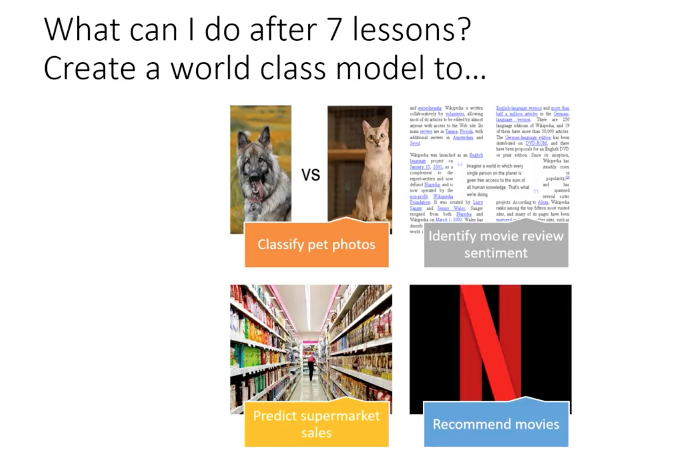
Currently, fastai supports 4 types of applications. They are -
- Computer Vision(images, videos)
- Natural Language Processing(Text)
- Tabular data(SQL like) and
- Collaborative filtering(recommendation systems).
Choosing Datasets -
We should choose well known academic datasets, we can get SOTA results, we can benchmark our model against them. our data is Oxford IIIT Pets data, With 37 distinct categories of pets, 25 dogs and 12 cat breeds.
Why not a simple cat vs dogs problem?
over the years it has become too easy we are getting accurate results without any fine-tuning. So this little harder problem this time.
The fastai library will automatically download all datasets for you.
Here is a dataset page for your reference.
Getting the data
path = untar_data(URLs.PETS)
URLs is a class from fastai. datasets, we imported it as from fastai import *
PETS is a string constant with the path as ‘https://s3.amazonaws.com/fast-ai-imageclas/oxford-iiit-pet’
what does untar_data do?
help(untar_data)
Help on function untar_data in module fastai.datasets:
untar_data(url:str, fname:Union[pathlib.Path, str]=None, dest:Union[pathlib.Path, str]=None)
Download url if doesn’t exist to fname and un-tgz to folder dest
the fname field is a union of path lib. Path type or str(either of) and it defaults to None.
The first time when you are running a notebook it will download data and untar it. just once.
Similarly, dest is a destination type. if not specified data will get saved in parent dir inside folder ‘oxford-iiit-pet’
Alternatively, you can use
?untar_data
or
??untar_data
to get more details about the particular function.
It will return the path object, which is an object-oriented filesystem path from python3 pathlib library.
It offers several methods to list or retrieve files.
pathlib - ‘/’ operator
path_anno = path/'annotations'
‘/‘ (slash) operator is python 3 operator which is part of the pathlib library.
How our labels look like?
Machine learning label refers to things we are trying to predict.
if we see the file path contains labels, we need a way to extract labels from the file path and link it to that image.
fnames = get_image_files(path_img)
fnames[:5]
[PosixPath('images/Abyssinian_1.jpg'),
PosixPath('images/Abyssinian_10.jpg'),
PosixPath('images/Abyssinian_100.jpg'),
PosixPath('images/Abyssinian_101.jpg'),
PosixPath('images/Abyssinian_102.jpg')]
Regular expressions
we can use a regular expression by importing regular expression ‘re’ package in python, to do this.
Regular expressions are a way to search a string in the text using pattern matching methods.
pat = r'/([^/]+)_\d+.jpg$'
Let’s deconstruct this regex pattern, /([^/]+)_\d+.jpg$ by reading it backward:
| Expression | Explanation |
|---|---|
$ |
end of search |
.jpg |
last chars to be found in the search string, also right file format checking |
\d |
numerical digits, ‘+’ sign denotes can be one or more of them |
_ |
should come before the start of digits |
() |
denotes a group of characters |
[] |
denotes another subgroup if characters in the previous group |
^/ |
‘^’ denotes negation, so ‘+’ says all other chars except ‘/’ |
( [ ^/ ] + ) |
searches all characters except ‘/’ |
/ |
first ‘/’ in regex says, end of search |
r |
The string should be a raw string. Otherwise, \d would have to be written as \\d so that Python doesn’t interpret it to be a special character. |
So, this regex pattern will give us a string
/Abyssinian_1.jpg
considering the search string was
PosixPath('images/Abyssinian_1.jpg')
Further, by using the fact that the actual name of the breed is in the first parenthesized group of the regular expression, the actual breed name
Abyssinian
can be obtained by using ‘.group(1)’ wherever the search on the regular expression is performed.See this for details.
credits @dreambeats
See this blog post to understand this regular expression in detail. The python documentation has a tutorial on regular expressions. RegexOne provides a simple interactive intro to regular expressions.
Loading the data
Loads the train, val & test data and applies transformations.
data = ImageDataBunch.from_name_re(path_img, fnames, pat, ds_tfms=get_transforms(), size=224)
There is a class called ImageDataBunch from fastai.vision.data, which will hold all the data you need an i.e train, val sets.
If you want to check from where particular class or function came from just type
ImageDataBunch
It will show you the hierarchy of modules where it has been defined.
fastai.vision.data.ImageDataBunch
To open up class documentation and source use doc function
doc(ImageDataBunch)
will open up the documentation page for you. Click on Show in docs button
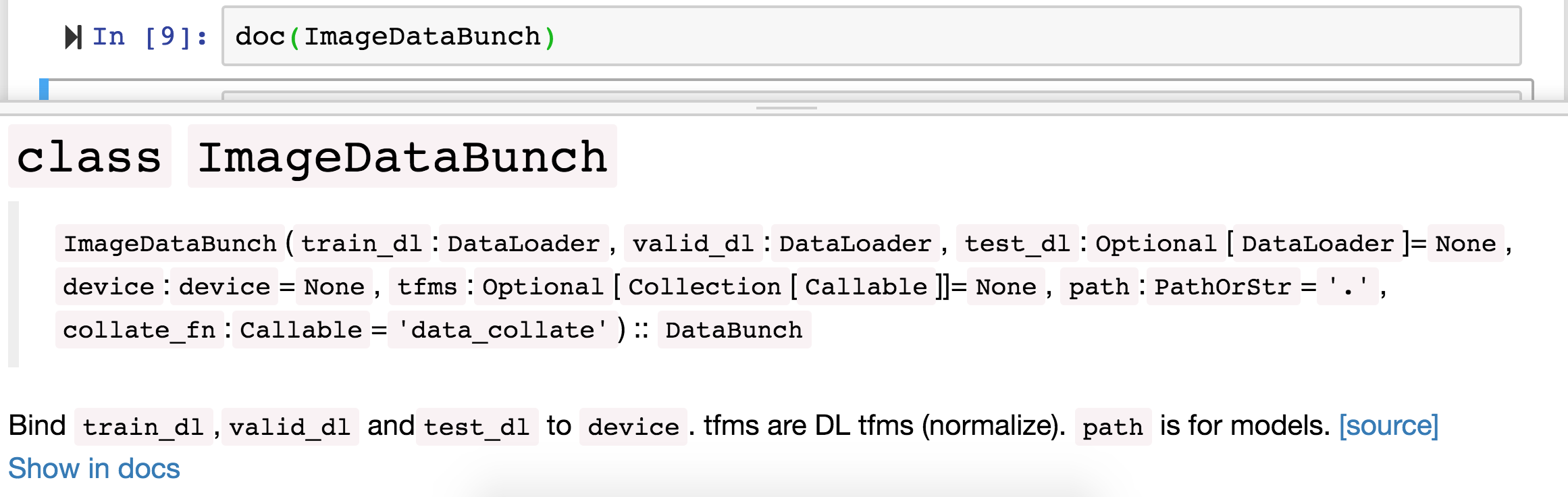
Below is how documentation looks on docs.fast.ai
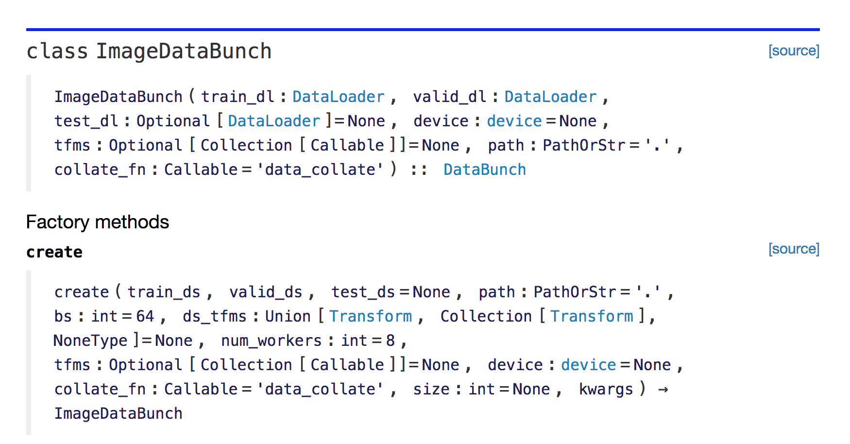
You can click on the source button to go to the python source code.
Transformations
ds_tfms are transformations that we will be applying to images on the fly. transforms also changes all the image sizes to 224 X 224 since on these sizes our architecture resnet34 has been trained on. Also, all the images get centered, cropped and zoomed a little bit by transformation functions.
from_name_re() is a factory method to extract labels using regular expressions.
Question: Why is normalization important?
data.normalize(imagenet_stats)
The pixel values of images range from 0 to 255. Images generally contain 3 color channels (Red, Green, and Blue). Sometimes some channels will be bright, some might be dull. Some might vary so much and some might not vary at all. It helps to train a model if all those 3 channels have got pixel values with a mean of 0 and a standard deviation of 1. Normalization simply does that. For more info
Advice: If you have trouble while training a model one thing to verify is that whether you have normalized the data properly.
Since we are using a pre-trained model on ImageNet, then the normalization that was used to pre-train ImageNet has to be applied to the new data (pets).
Question: As GPU mem will be in power of 2, doesn’t size 256 sound more practical considering GPU utilization compared to 224?
The brief answer is that the models are designed so that the final layer is of size 7 by 7, so we want something where if you go 7 times 2 a bunch of times (224 = 72222*2), then you end up with something that’s a good size.
Looking at the data
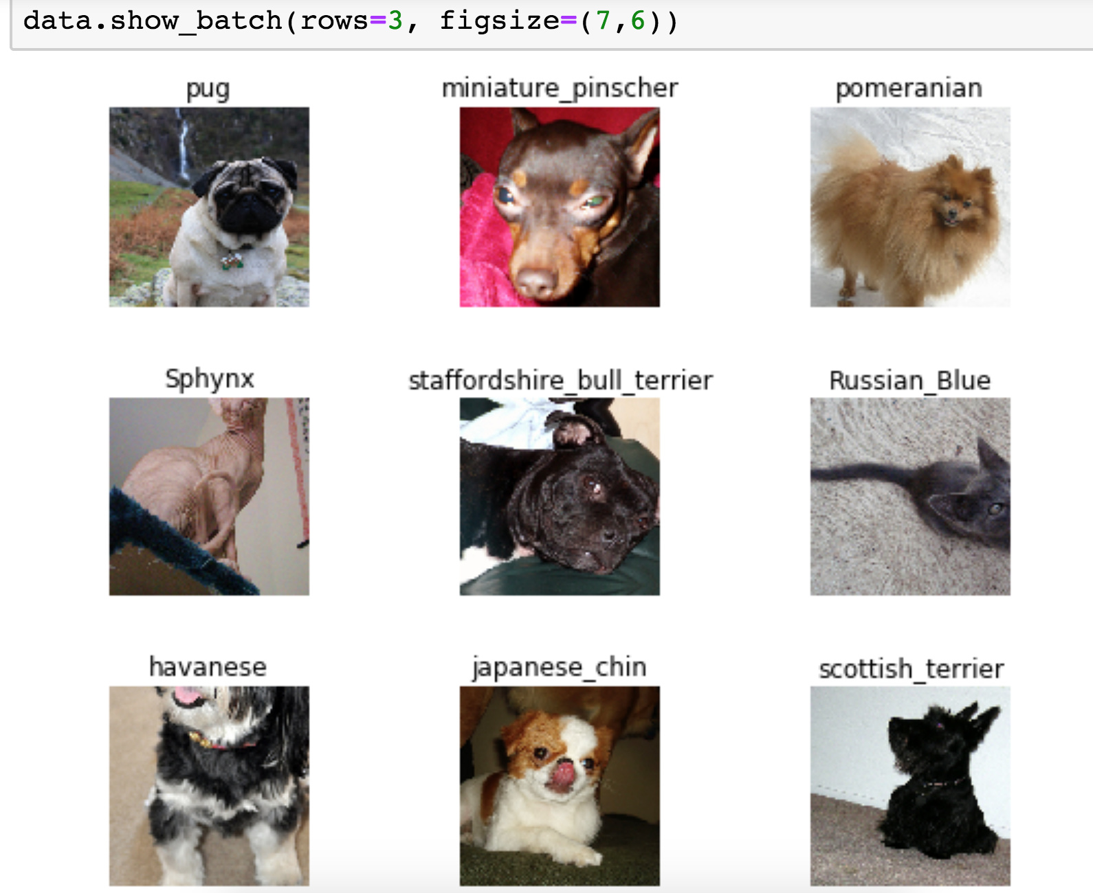
It’s really important to look at your data and check if everything looks fine.
Sometimes images can have text on it, or they might be occluded by some other object, or some of them might be rotated in odd ways.
Looking at the labels
ImageDataBunch gives
data.classes
that lists down all the classes you have got.
also, it is important to check the total number of classes by
len(data.classes)

Yes, we have indeed 37 classes in oxford pet dataset.
the data.c property also gives the number of classes.
Training a model using resnet architecture
resnet works well with almost all the image classification problems, you need to just care about how big architecture is.
In resnet34, 34 signifies the number of layers in the model architecture. we will also use resnet50 ahead.
Learner:
learn = create_cnn(data, models.resnet34, metrics=error_rate)
create_cnn method resides in fastai.vision.learner class.
In fastai, the model is trained by a learner, create_cnn takes few parameters, first the DataBunch data object, then model resnet34, the last thing to pass is the list of metrics.
When you call create_cnn first time, it downloads resnet34 pre-trained weights.
Pre-trained means this particular model has been already trained for the particular task, and that task is it is been trained on 1 and half million pictures of 1000 different categories of objects like plants, animals, people, cars, etc. using image dataset called Imagenet.
So we don’t necessarily start with a model that knows nothing about images, but we start with knowledge of images of 1000 categories.
Applying One Cycle Policy
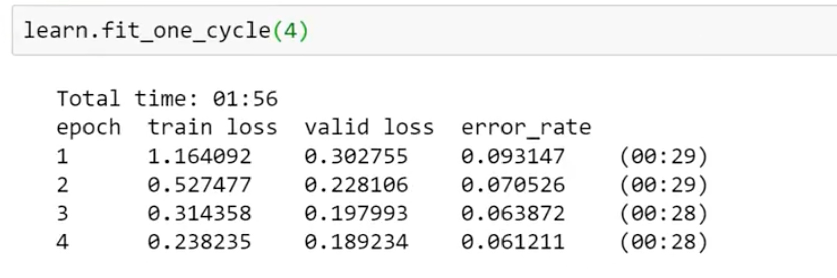
learn.fit_one_cycle(4)
fit_one_cycle method fits a model following one cycle policy.
It accepts cycle_len which is an integer describing how many times you want to pass through the complete dataset. Each time the model sees a picture, it keeps getting better. It gonna take a lot of time. But if you show images too many times, the model will learn to recognize that image alone. In machine learning, this is called overfitting. (memorizing).
max_lr is maximum learning rate, moms are momentum and wd is weight decay we will learn about all these parameters in subsequent lectures.
We can tune cycle_len as much as we want till we get better results. For now, 4 is a pretty good number. If you see an error_rate column in the output. after 4 epochs(4 times complete pass-through data) we have got a 6% error. 94% accuracy means we have identified correctly 94% pictures of dogs and cats among all the images.
The total time taken to fit this model is under 2 mins.
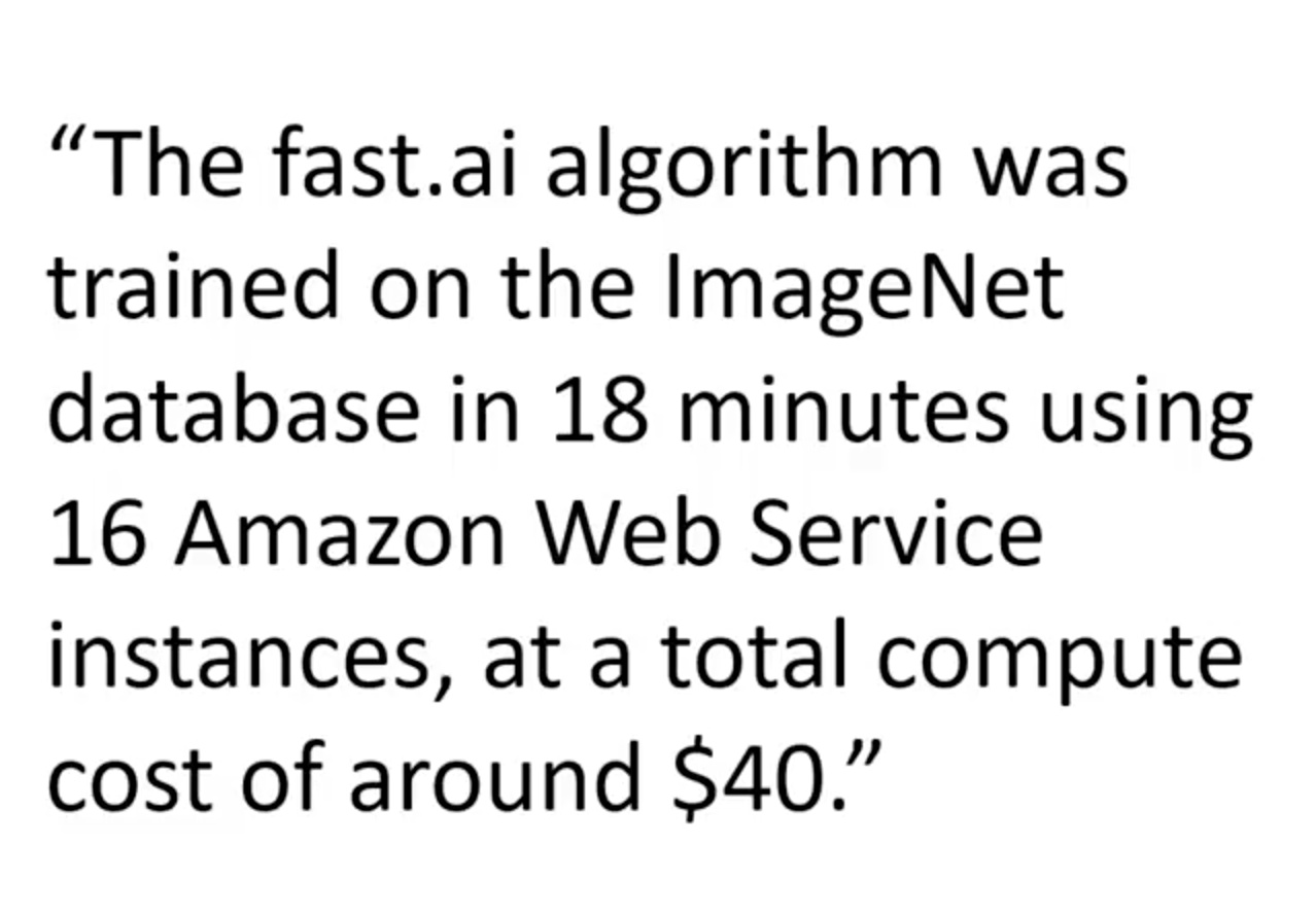
original Paper benchmark
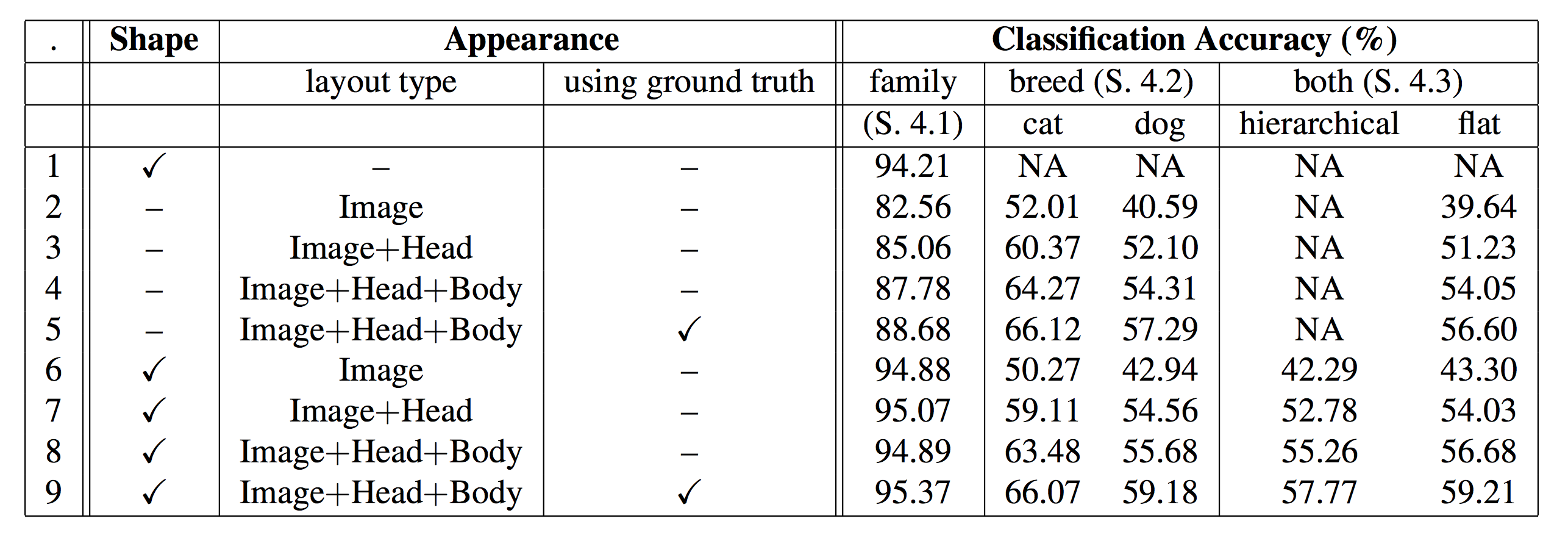
In 2012 accuracy on this dataset was at 59.21% and now in 2018 with just 3 lines of code, we got 94% i.e just 6% error.
This shows how far we have come with deep learning, and particularly with Pytorch and fastai.
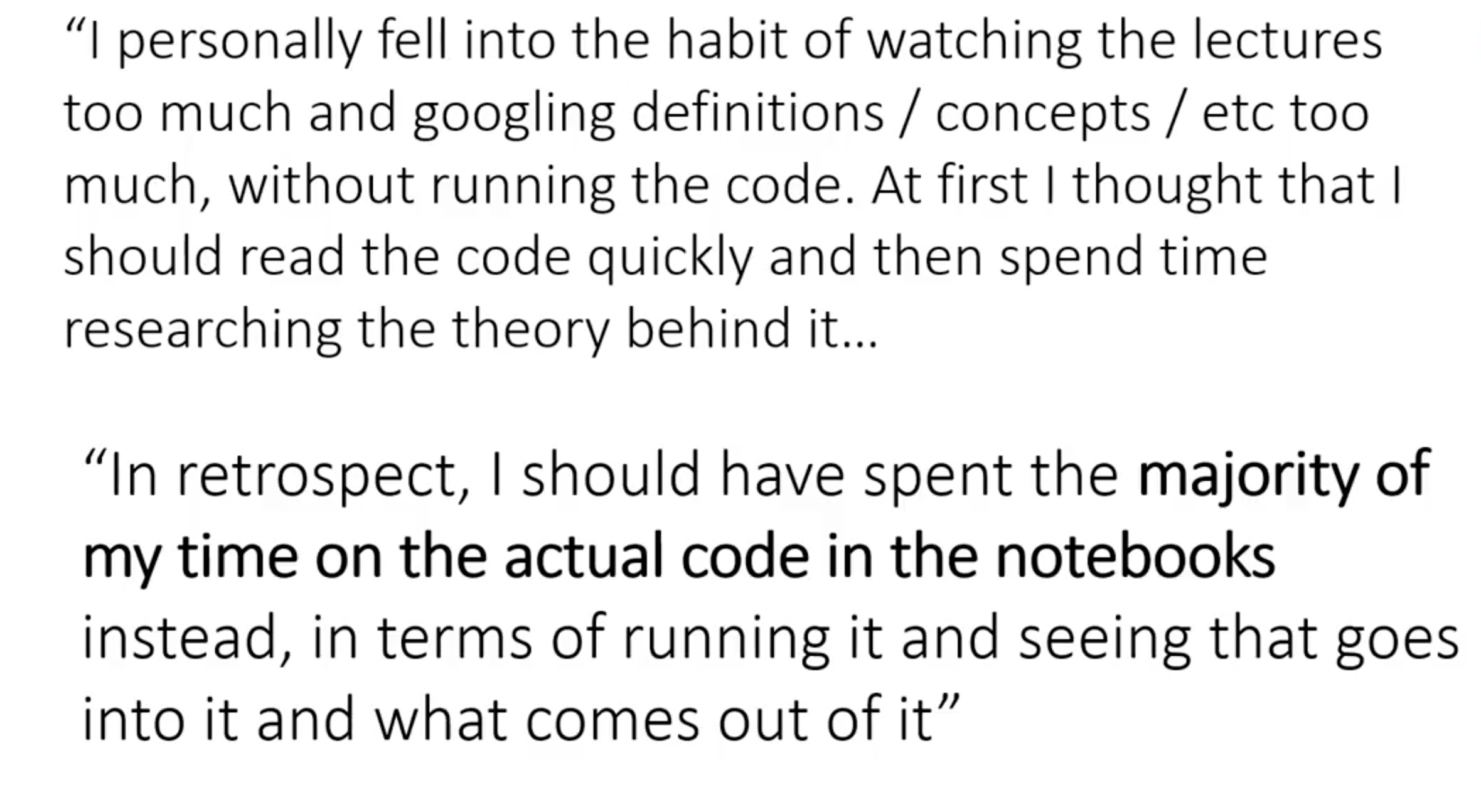
PLEASE Run the Code!!!
About the fastai library
The reason we can achieve these results quickly is due to the fastai library. Even though it’s pretty new, it’s already getting a lot of traction. Almost all major cloud providers have fastai preinstalled. Researchers have started using it. So, understanding fastai software thoroughly is going to take you a long way. The best way to dig into the fastai library is to go through the fastai documentation
Keras
How does the fastai library compare to any other library?
There is only one library that makes deep learning easy to use just like fastai is Keras.
It’s an excellent piece of software. we used it for 1st version of the course till we switched to PyTorch.
If you look at last year’s fastai course example Dogs Vs. Cats compared to Keras.
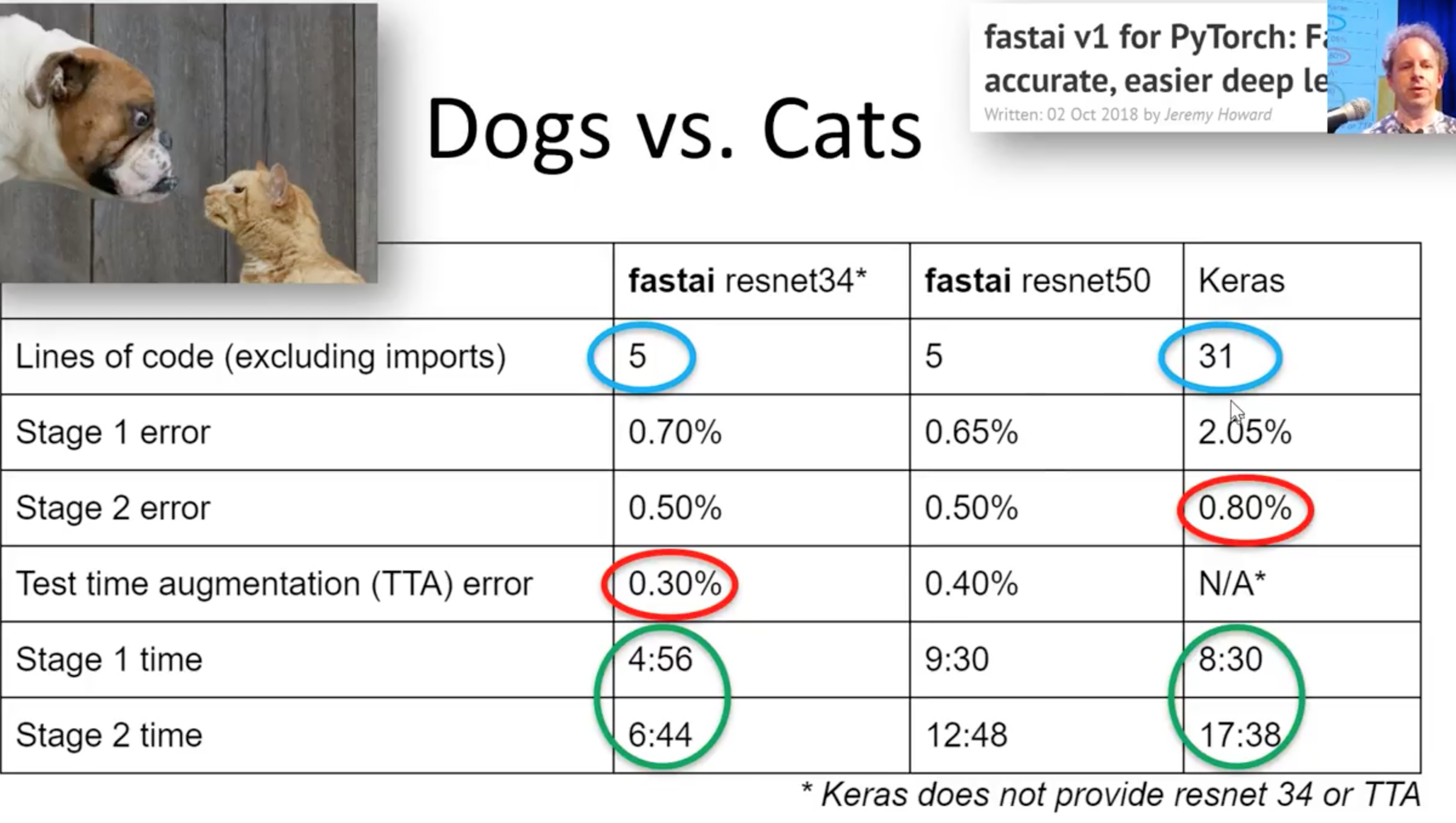
- We have got almost less than half error on the validation set (see fastai TTA error vs. stage 2 error Keras)
- Training time is also almost half.
- The number of lines of code with fastai is the way to less compared to that of Keras.
Those 31 lines of code in Keras forces you to take a lot of decisions, tuning hyperparameters, adjusting configurations. It expects you to know all those things which can get you best practice results.
Versus these 5 lines of code in fastai takes care of most of the best practice methods for us already.
This will make fastai very useful library for you not just for learning but for putting software in productions.
About forums
To learn more about the fastai course and library, there is one more place forums.
You can ask questions about lessons, doubts. There are different categories, you can talk about current research papers, applications and general deep learning, etc.
While asking questions check once whether they have been already asked before.
Make sure you provide enough information about the environment you are using, the changes you made and complete error screenshots so that it can be well understood to answer.
Advice: Just get involved. Everybody here once started not knowing things.
Examples of cool projects done by fastai students:
Pick up your passion project and work on it.
- Karthik created Envision tool to empower visually impaired people to live more independently.
- Melissa Fabros won a $1million challenge of kiva micro-lending organization to detect black women and men faces accurately, which much prominent software failed to do.
- Alexandre Cadrin identified the overfitting issue in MIT’s deep learning model to detect pneumonia in medical x-ray images due to his domain knowledge in Radiology and fastai DL course.
- Christine Payne developed Clara: A Neural Net Music Generator
- Sara Hooker, a Google brain resident works on detecting illegal cutting of trees in the Amazon rainforest by detecting chainsaw noises using old recycled cellphones.
- Stanford’s DawnBench Competition
- @helena created beautiful art using GANs
- Brad Kenstler used Style Transfer to Draw Kanye using Captain Picard’s Face.
- A Splunk engineer developed an algorithm to detect fraudulent behavior using biometrics.
- Not hotdog app was Emmy nominated.
Back to coding
Question: Why resnet and not inception architecture??
Resnet is Good Enough. ![]()
See the results below from Stanford’s DAWNBench Competition all top 4 teams used resnet.
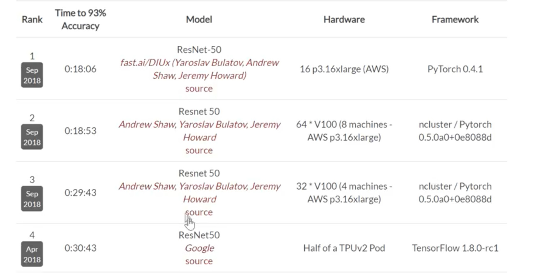
You can consider different models for different use cases.
For example, if you want to do edge computing, mobile apps, Jeremy still suggests running the model on the local server and port results to the mobile device. But if you want to run something on the low powered device, there are special architectures for that.
Inception is pretty memory intensive.
fastai wants to show you ways to run your model without much fine-tuning and still achieve good results.
The kind of stuff that always tends to work. Resnet works well on a lot of image classification applications.
Training model
learn.fit_one_cycle()
Training means creating a set of weights. i.e, finding a set of coefficients in case of linear or logistic regression.
Searching parameters that fit well to the data.
Saving model weights
This step is very important as you may need to reload your weights next time you run the code.
learn.save('stage-1')
this will save the model as .pth format, which is Pytorch’s default serialization method.
Models will get saved into your local dir in /models folder
Since different model’s weights should be saved separately we use local directories instead of a global one.
If we want to play around more with hyperparameters, we should save weights.
Analyzing results
It’s important to see what comes out of our model. We have seen one way of what goes in, now let’s see what our model has predicted.
Jeremy says this is the other thing you need to get good at.
interp = ClassificationInterpretation.from_learner(learn)
ClassificationInterpretation
This class has methods for creating confusion matrix as well as plotting misclassified images.
We are going to use this class called ClassificationInterpretation for this.
and factory method from_learner(learn).
Remember to pass learn object, learn object knows 2 things, data, and model.
The model here is not just the architecture but a trained model with weights.
We need to interpret that model, we pass in the learner of a ClassificationInterpretation object.
Plot top losses
We will learn about loss functions shortly. But the idea is loss function tells you how good was your prediction compared to the ground truth.
Specifically, that means if you predicted one class of cat with great confidence.
For example, if you confidently predicted this is a Berman cat, but it was wrong. It was a Ragdoll cat. Then it is going to have a very high loss because you were very confident about the wrong answer.
So by plotting the top losses, we are going to plot images that were most confident about the prediction but were wrong.
interp.plot_top_losses(9, figsize=(15,11))

If you see the title of each image, it prints out 4 things.
If you want to know what are they doc() function is your way to go.
doc(interp.plot_top_losses)
These are a prediction, actual, loss, the probability of actual class.
Don’t be afraid to look at source code.
If you are a python programmer, you will find this source code of fastai very easy to read.
This is the most important interpretation tool that we have. Because it lets us see the things that model has got wrong.
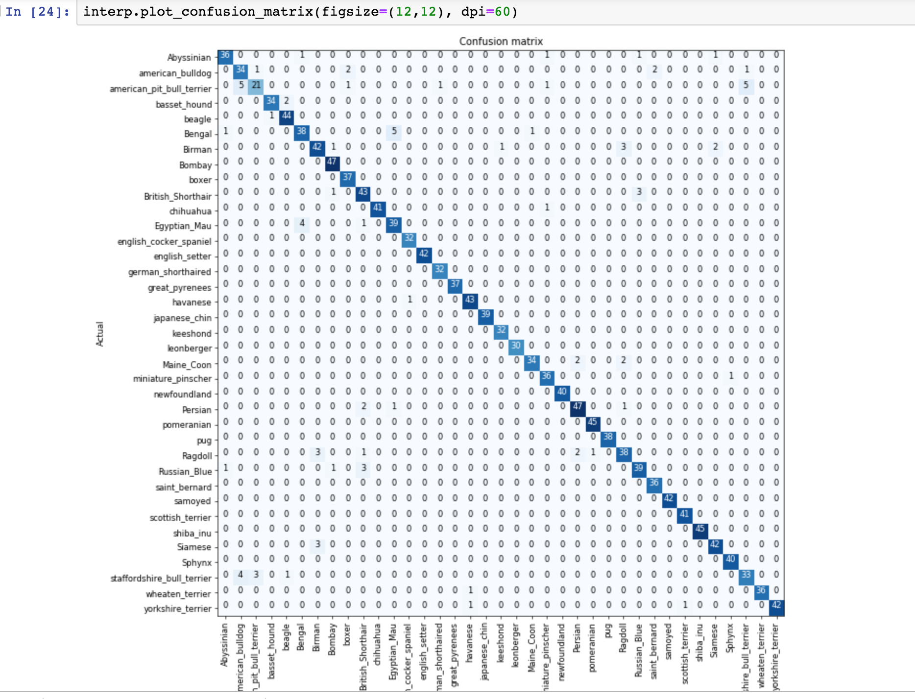
Confusion Matrix:
It shows you for every actual type of dog or cat, how many times the model predicted to be of that dog or cat.
Because it’s pretty accurate this time it shows darker diagonal line, with little lighter numbers for some other wrong combinations.
If you have got lots of classes, don’t use a confusion matrix. instead, use named function by fastai called most_confused().
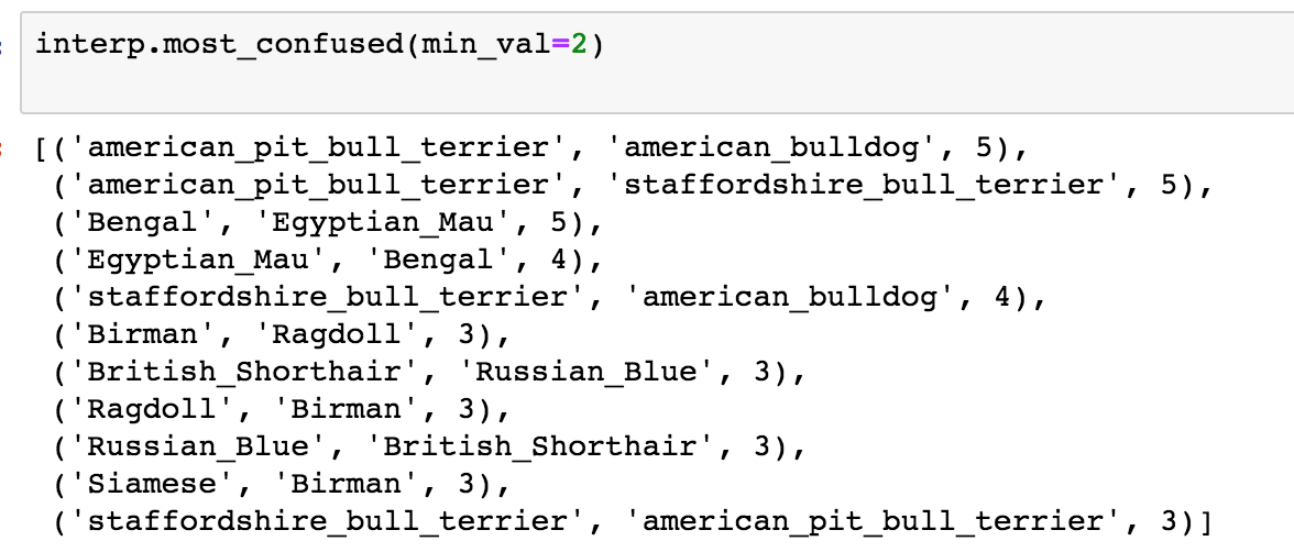
Most confused categories
most_confused() function will simply grab out of the confusion matrix the most confusing combinations of predicted and actual categories, that it got wrong most often.
Making model Better
So how do we make the model better?
Unfreezing, fine-tuning and learning rates
We can make our model better by Fine-tuning
So far we have fitted 4 epochs and it ran pretty quickly. Why is that so? Because we used a little trick (called transfer learning).
These deep learning models have many layers. We will learn later about what layers are. But for now, understand that it goes through a lot of computations.
What did we do?
We added a few extra layers at the end of architecture, and we only trained those. we left most of the early layers as they were. This is called freezing layers i.e weights of the layers. So that was fast.
If we want to build a model, that is quite similar to the original retrained model, in this case, similar to Imagenet data that works pretty well.
What do we want to do?
To go back and train the whole model. So this is why we always use this 2-state process.
- when we call fit or fit_one_cycle() on a create_cnn, it will just fine-tune these extra layers at the end, and run very fast.
- It will never overfit, but to get it good, you have to call.
learn.unfreeze()
unfreeze() says train the whole model.
Then again we have to call fit_one_cycle() but the error we got now is much worse.
Why has that happened?
To understand why? we have to know what is going on behind the scenes.
Let’s start by train to get an intuitive understanding of what is happening behind the scenes.
and we will do this by looking at pictures.
Visualizing layers of the convolutional model.
Visualizing and understand Convolutional models by Matthew D. Zeiler and Rob Fergus.
This paper shows how can you visualize layers of a convolutional network.
The convolutional neural network will learn about mathematically about what the layers are.
There are Red, Green, and Blue pixel values with numbers ranging from 0 to 255.
These values go into simple computation in the first layers and then it’s output goes into a computation of the second layer, the result of that goes to a third layer and so on.
These layers can go up to 1000 layers of a neural network.
Resnet34 has 34 layers, resnet50 has 50 layers.
But let’s look at layer 1 first.
There is a very simple computation called convolution. we will learn about it shortly.
In layer 1,
We can visualize these specific coefficients/parameters by drawing them like the picture.
There can be few dozens of them but we will look at random 9 filters.
Here is the example of 9 actual coefficients or parameters.
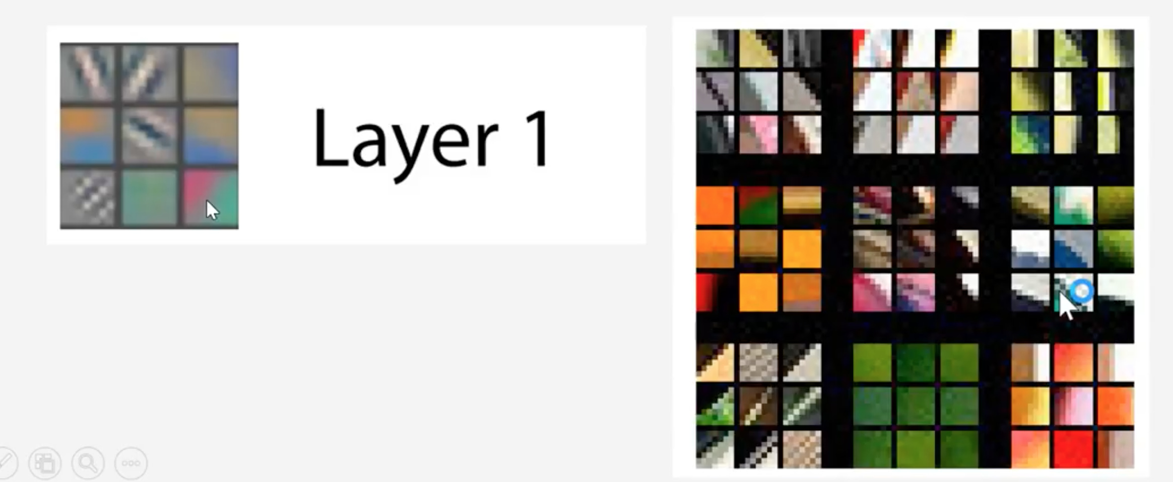
These operate on a group of the pixel that is next to each other.
1st and second columns in a 1st row find if there is a little diagonal line in either direction.
3rd column shows it finds gradients that go from yellow to blue and vice versa also pink to green in those directions and so forth.
That’s a very simple convolution that can find little lines.
That’s layer 1 of the Imagenet pre-trained convolutional neural network.
Layer 2
takes the result of those filters and does the second level of computation.
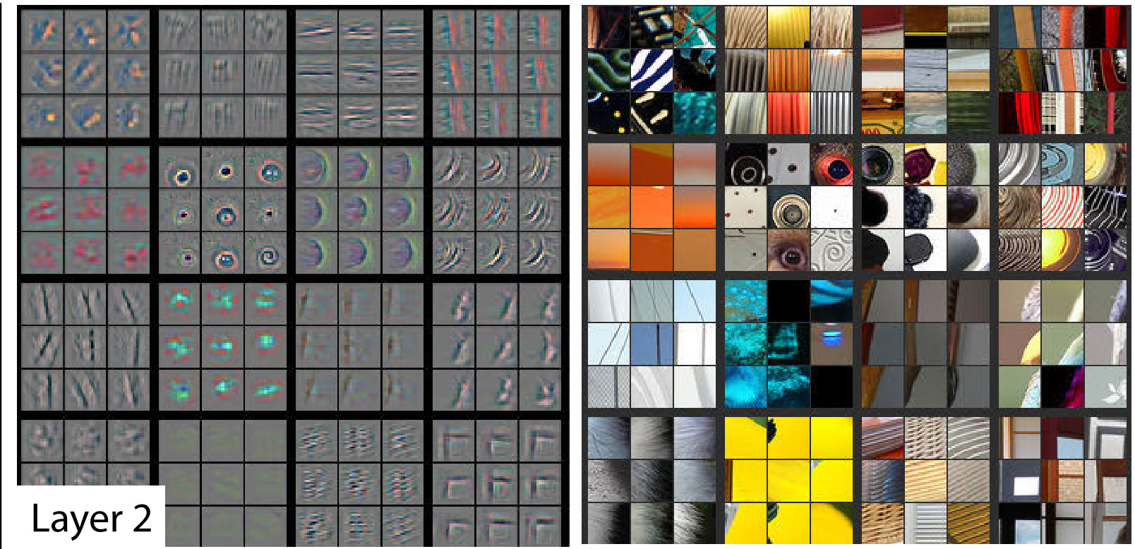
If you look at the bottom rightmost image on the left side, if looks for corners of windows,
or in 3rd column 2nd row image says it found righthand curves
or 2nd column 2nd row it learns to find little circles.
So if in layer 1 we could just find one line, by layer 2 we can find shapes.
If you look at these 9 images in actual photos, which activated these filters.
So this filter/math function was good at finding window corners or stuff like that.
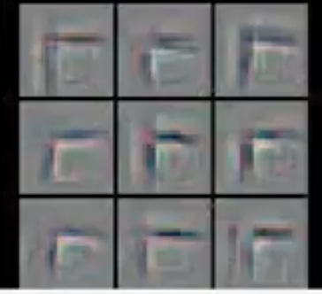
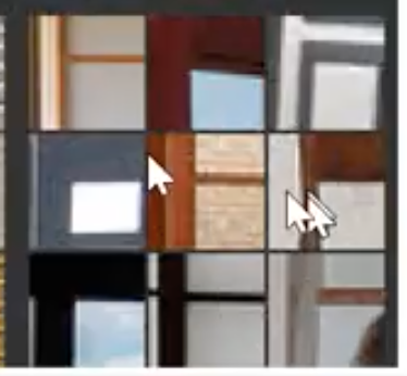
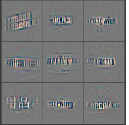
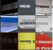
Layer 3
It can find combinations of lines and shapes.
We can find repeating patterns of 2-D objects or lines that join together.
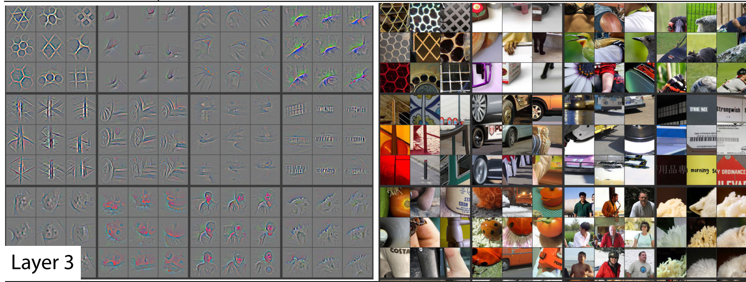
Here it finds edges of fluffy things at the bottom right corner.
Also, Geometric patterns at the top left the corner.
Also we can see below repeated pattens of text sometimes windows also activated these filters.
Layer 4
picked all the stuff from layer 3 and combined them and found dog faces or bird legs.
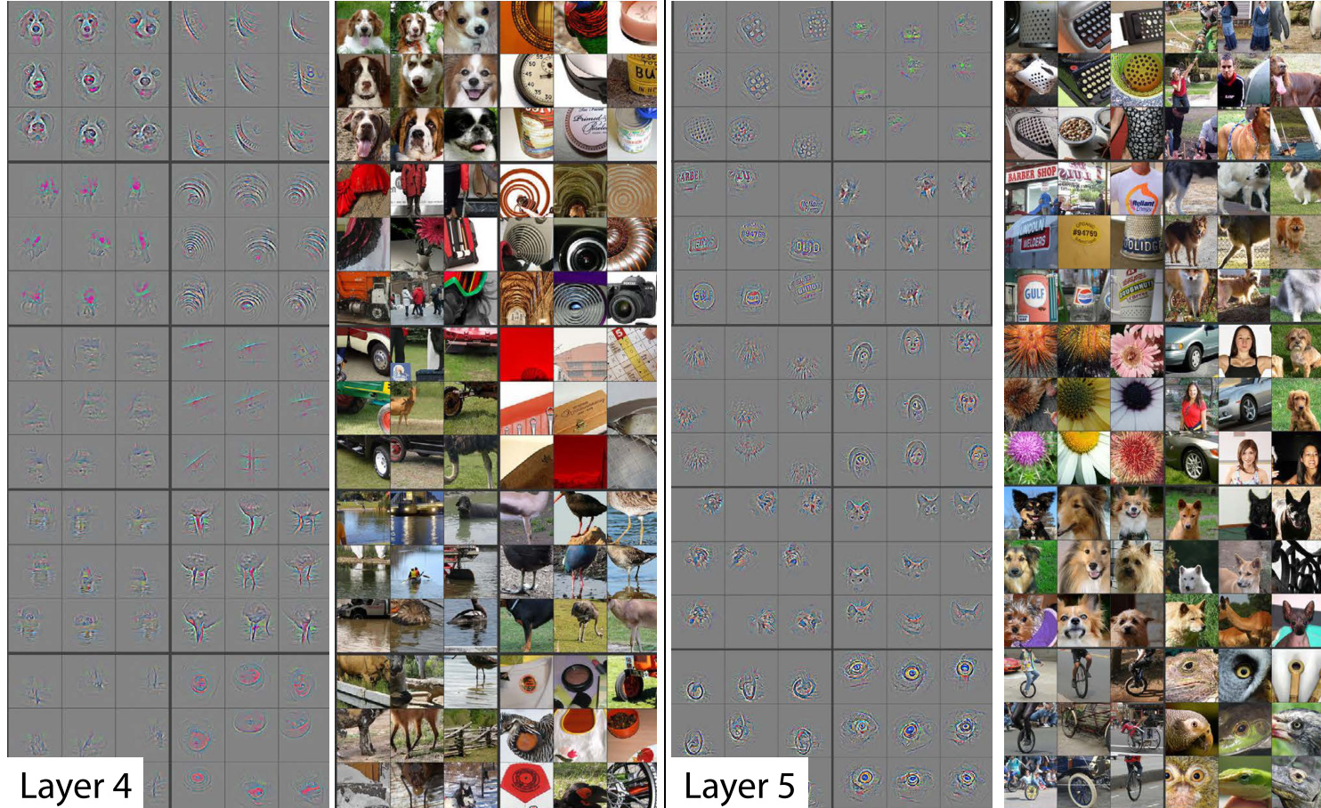
layer 5
It can find eyeballs of birds /lizards or faces of a particular breed of a dog.
By the time it gets to layer 34, the final layer (in case of resnet34 architecture), it would have learned to visualize a particulate breed of cat or dog accurately.
This is kind of how it works.
So when we first trained that specific model
Now we are fine-tuning we are saying let’s change all of that. We will keep them where they are but let’s see if we can make them better.
So, it’s very unlikely if we can make layer 1 features better. It’s very unlikely that the definition of the diagonal line will ever change for dog or cat breed or any kind of image for that matter versus the Imagenet data it was originally trained on.
But the last layer considers 5th here. we would like to change the faces of dogs as in our dataset.
So intuitively you can understand that different layers of convolutional neural net represent different levels of semantic complexity.
So this is why out attempt of fine-tuning this network didn’t work as we expected.
By default, it trains all the layers at the same speed. So it updates the things that look like diagonal lines or circles the same as it updates the things that have specific details of a particular dog or cat breed. So we have to change that.
To change that we need to go back to where we were before. We just broke this model.
Load the weights
Let’s load the weights of the model we saved earlier as stage-1.
So now our model is back to where it was before we killed it.
Find the learning rate.
Let’s run the learning rate finder. We will learn about it next week.
This is the thing that figures out what is the fastest I can train this neural network without making it zip off the rails and get blown apart.
learn.lr_find()
we can plot the results about lr_find
learn.recorder.plot()
plt.title("Loss Vs Learning Rate")
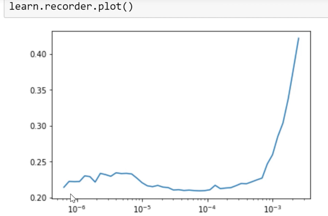
This will plot the result of our LR finder and what this shows you is the key parameter called a learning rate. The learning rate says how quickly are we updating the parameters in our model. The x-axis one here shows me what happens as I increase the learning rate. The y-axis shows what the loss is. So you can see, once the learning rate gets passed 10-4, our loss gets worse. We can check this by pressing shift+tab here, our learning defaults to 0.003 = 10-3. So you can see why our loss got worse. Because we are trying to fine-tune things now, we can’t use such a high learning rate. So based on the learning rate finder, we tried to pick something well before it started getting worse. So Jeremy decided to pick 1e-6. But there’s no point training all the layers at that rate because we know that the later layers worked just fine before when we were training much more quickly. So what we can do is we can pass a range of learning rates to learn.fit_one_cycle. And we do it like this:
learn.unfreeze()
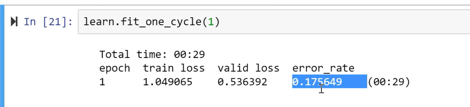
learn.fit_one_cycle(2, max_lr=slice(1e-6,1e-4))
You use this keyword in Python called slice and that can take a start value and a stop value and basically what this says is train the very first layers at a learning rate of 1e-6, and the very last layers at a rate of 1e-4, and distribute all the other layers across that between those two values equally.
learning rates after unfreezing
[1:25:20]
The basic rule of thumb is after you unfreeze (i.e. train the whole thing), pass a max learning rate parameter, pass it a slice, make the second part of that slice about 10 times smaller than your first stage. Our first stage defaulted to about 1e-3 so it’s about 1e-4. And the first part of the slice should be a value from our learning rate finder which is well before things started getting worse. So you can see things are starting to get worse maybe about here
So we picked something that’s at least 10 times smaller than that.
If we do that, then we get a 0.0578 error rate. So we got down from 6.1% to a 5.7% error rate, So that’s about 10% point relative improvement.
Jeremy would perhaps say for most people most of the time, these two stages are enough to get pretty much a world-class model. You won’t win a Kaggle competition, particularly because now a lot of fastai alumni are competing on Kaggle and this is the first thing that they do. But in practice, you’ll get something that’s about as good in practice as the vast majority of practitioners can do.
ResNet50
[1:26:56]
data = ImageDataBunch.from_name_re(path_img, fnames, pat, ds_tfms=get_transforms(),
                                   size=299, bs=bs//2).normalize(imagenet_stats)

learn = create_cnn(data, models.resnet50, metrics=error_rate)
We can improve it by using more layers and we will do this next week but by basically doing a ResNet50 instead of ResNet34. And you can try running this during the week if you want to. You’ll see it’s the same as before, but I’m using ResNet50 instead of resnet34.
What you’ll find is it’s very likely if you try to do this, you will get an error and the error will be your GPU has run out of memory. The reason for that is that ResNet50 is bigger than ResNet34, and therefore, it has more parameters and uses more of your graphics card memory, just totally separate from your normal computer RAM, this is GPU RAM. If you’re using the default Salamander, AWS, then you’ll be having a 16G of GPU memory. The card Jeremy uses most of the time has 11G GPU memory, the cheaper ones have 8G. That’s kind of the main range you tend to get. If yours have less than 8G of GPU memory, it’s going to be frustrating for you.
It’s very likely that if you try to run this, you’ll get an out of memory error and that’s because it’s just trying to do too many parameter updates for the amount of RAM you have. That’s easily fixed. ImageDataBunch constructor has a parameter at the end bs i.e a batch size. This says how many images do you train at one time. If you run out of memory, just make it smaller. bs=48 works for Jeremy on 8G card if it doesn’t work for you decrease the batch size to 32 or less than that.
It’s fine to use a smaller batch size. It might take a little bit longer. That’s all. So that’s just one number you’ll need to try during the week.
learn.fit_one_cycle(8, max_lr=slice(1e-3))
Again, we fit it for a while and we get down to 4.4% error rate. So this is pretty extraordinary. I was pretty surprised because when we first did in the first course, these cats vs. dogs, we were getting somewhere around 3% error for something where you’ve got a 50% chance of being right and the two things look different. So the fact that we can get a 4.4% error for such a fine grain thing, it’s quite extraordinary.
Jeremy fitted it some more, it went to 4.35% that’s a tiny improvement. Resnet50 is a pretty good model.
Interpreting the results
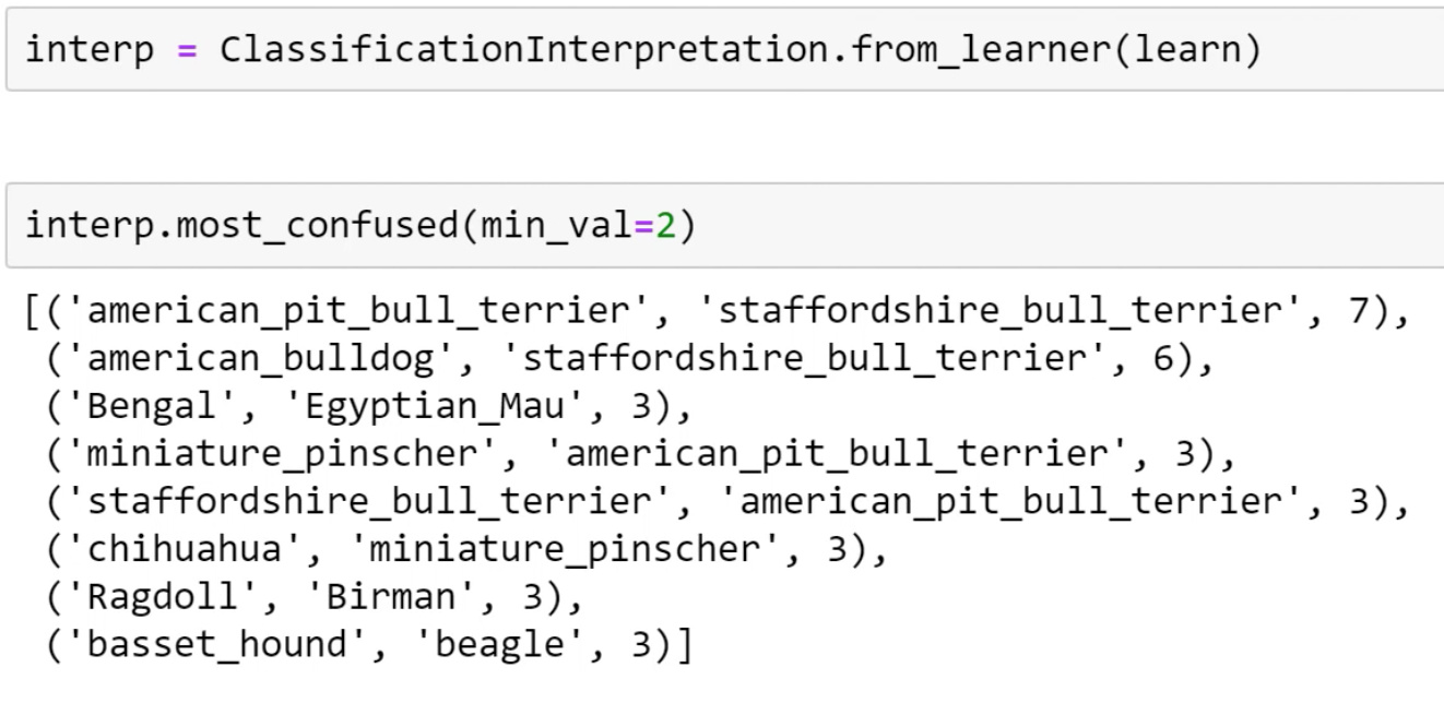
We can call the most_confused here and we can see the kinds of things that it’s getting wrong. Depending on when we run it, we are going to get slightly different numbers, but we’ll get roughly the same kind of things. So quite often, Jeremy finds the Ragdoll and Birman are things that it gets confused. Jeremy had never heard of either of those things, so he looked them up and found a page on the cat site called “Is this a Birman or Ragdoll kitten?” and there was a long thread of cat experts arguing intensely about which it is. So Jeremy feels fine that his computer had problems.
Jeremy found something similar about pitbull versus Staffordshire bull terrier, apparently, the main difference is the particular kennel club guidelines as to how they are assessed. But some people think that one of them might have a slightly redder nose. So this is the kind of stuff where even if you’re not a domain expert, it helps you become one. Because I now know more about which kinds of pet breeds are hard to identify than I used to. So model interpretation works both ways.
Homework
[1:31]
So what Jeremy wants us to do this week is to run this notebook, make sure we can get through it, but then he really wants us to do is to get our image dataset and actually Francisco, who started language model zoo thread, is putting together a guide that will show us how to download data from Google Images so we can create our dataset to play with. But before Jeremy does that, he wants to show us how to create labels in lots of different ways because our dataset where we get it from won’t necessarily be that kind of regex-based approach. It could be in lots of different formats. So to show us how to do this, he’s going to use the MNIST sample. MNIST is pictures of hand-drawn numbers just because Jeremy wants to show us different ways of creating these datasets as below.
1. labels that are folders names
path = untar_data(URLs.MNIST_SAMPLE); path
path.ls()
['train', 'valid', 'labels.csv', 'models']
We can see there are a training set and the validation set already. So basically the people that put together this dataset have already decided what they want us to use as a validation set.
(path/'train').ls()
['3', '7']
There are a folder called 3 and a folder called 7. Now, this is a really common way to give people labels. It says everything that’s a three, we put that in a folder called 3. Everything that’s a 7, we’ll put in a folder called 7. This is often called an “ImageNet style dataset” because this is how ImageNet is distributed. So if we have something in this format where the labels are just whatever the folders are called, we can say from_folder.
tfms = get_transforms(do_flip=False)
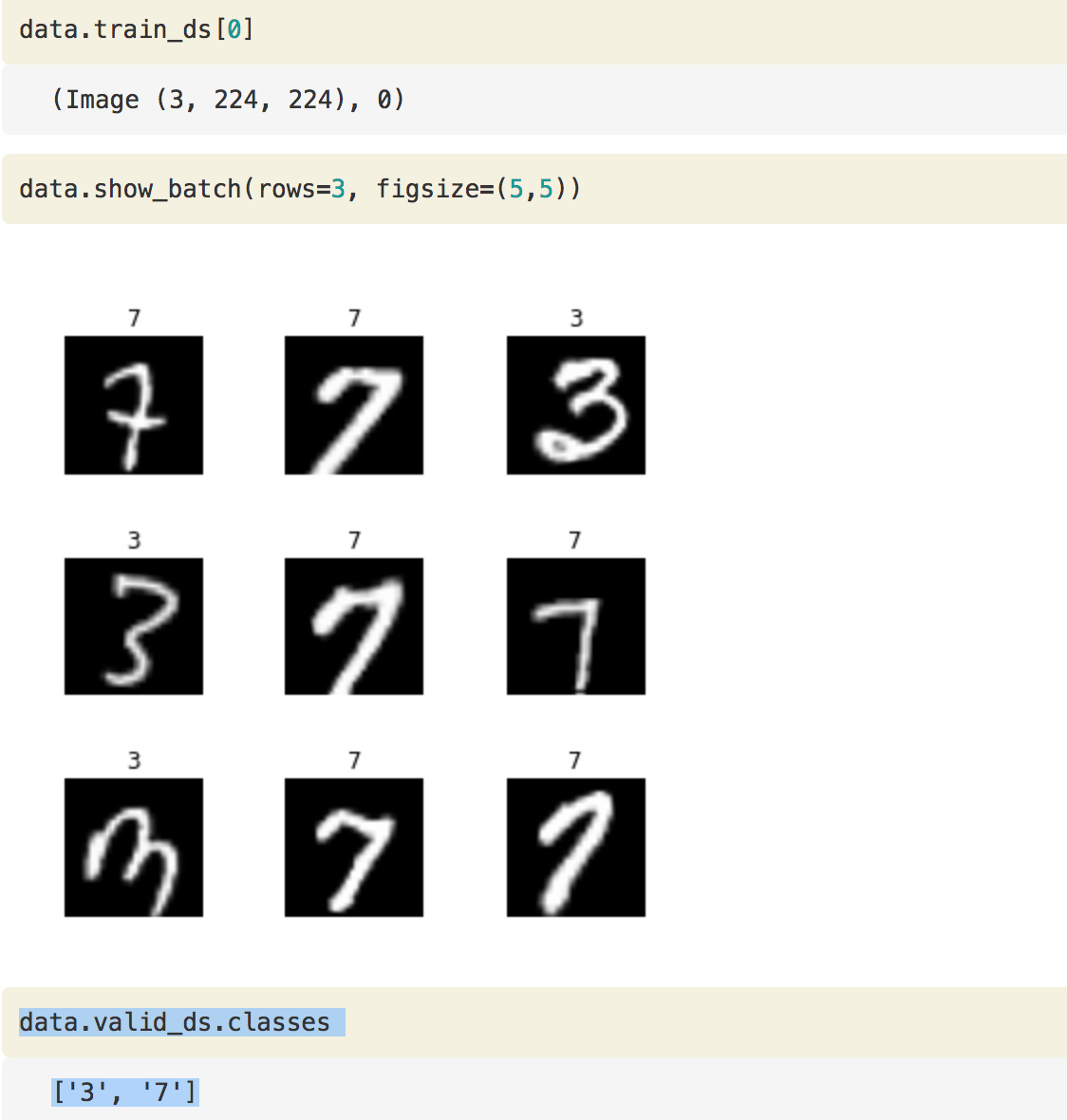
data = ImageDataBunch.from_folder(path, ds_tfms=tfms, size=26)
This will create an ImageDataBunch for us and as we can see it created the labels as well:
data.show_batch(rows=3, figsize=(5,5))
2. labels are in CSV file
[1:33:13]
Another possibility, and for this MNIST sample, we’ve got both, it might come with a CSV file that would look something like this.
df = pd.read_csv(path/'labels.csv')
df.head()
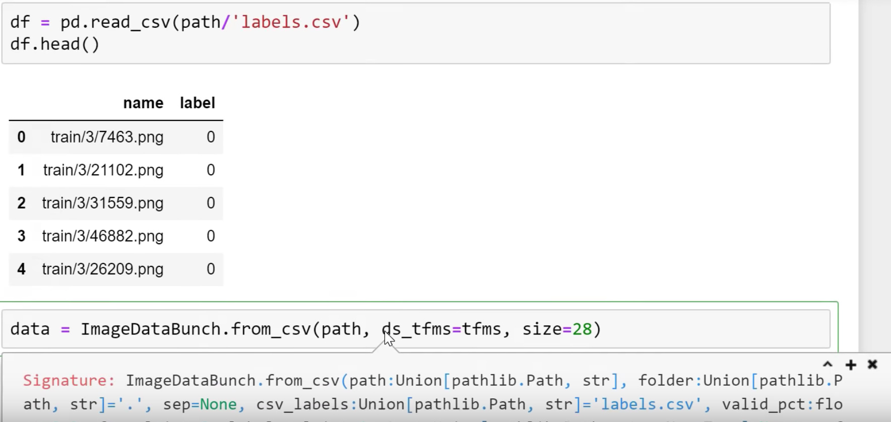
For each file name, what’s its label. In this case, labels are not three or seven, they are 0 or 1 which is it a 7 or not. So that’s another possibility. If this is how your labels are, you can use from_csv :
data = ImageDataBunch.from_csv(path, ds_tfms=tfms, size=28)
And if it is called labels.csv, you don’t even have to pass in a file name. If it’s called something else, then you can pass that filename in the csv_labels parameter.
data.show_batch(rows=3, figsize=(5,5))
data.classes
[0, 1]
3. Extracting labels using regular expressions
[1:34]
 fn_paths = [path/name for name in df['name']]; fn_paths[:2]

Out[ ]:

[PosixPath('/home/ubuntu/course-v3/nbs/dl1/data/mnist_sample/train/3/7463.png'), PosixPath('/home/ubuntu/course-v3/nbs/dl1/data/mnist_sample/train/3/21102.png')]
This is the same thing, these are the folders. But we could grab the label by using a regular expression. We’ve already seen this approach.
pat = r"/(\d)/\d+\.png$"
data = ImageDataBunch.from_name_re(path, fn_paths, pat=pat, ds_tfms=tfms, size=24)
data.classes
['3', '7']
4. Extracting labels from a function
[1:34:20]
Something more complex which is not ina simple file name or path we can create an arbitrary function that extracts a label from the file name or path. In that case, you would say from_name_func :
data = ImageDataBunch.from_name_func(path, fn_paths, ds_tfms=tfms, size=24,
label_func = lambda x: '3' if '/3/' in str(x) else '7')

data.classes
['3', '7']
5. Creating an array of labels and passing them as a list
[1:34:40]
If you need something even more flexible than that, you’re going to write some code to create an array of labels. So in that case, you can just use from_lists and pass in the array.
labels = [('3' if '/3/' in str(x) else '7') for x in fn_paths] labels[:5]
['3', '3', '3', '3', '3']

data = ImageDataBunch.from_lists(path, fn_paths, labels=labels, ds_tfms=tfms, size=24) data.classes
['3', '7']
So you can see there are lots of different ways of creating labels. So during the week, try this out.
Now you might be wondering how would you know to do all these things? Where am I going to find this kind of information? So I’ll show you something incredibly cool. You know how to get documentation:
doc(ImageDataBunch.from_name_re)
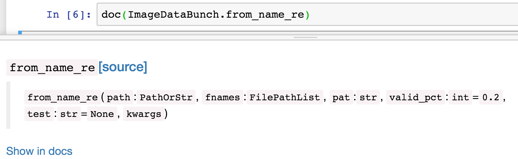
If you click on Show in docs link it pops up the documentation.
Every single line of code Jeremy just showed us, he took it this morning and he copied and pasted it from the documentation. So we can see here the exact code that he just used. So the documentation for fastai doesn’t just tell you what to do but step by step how to do it. And here is perhaps the coolest bit. If you go to fastai/fastai_docs on GitHub and click on docs/src.
All of the fastai documentation is just Jupyter Notebooks. In this case, Jeremy was using vision.data.ipynb.
We can download this repo. We can git clone this repo and if you run it, you can run every single line of the documentation yourself.
This is the kind of the ultimate example to Jeremy of experimenting. Anything that you read about in the documentation, nearly everything in the documentation has actual working examples in it with actual datasets that are already sitting in there in the repo for us. So we can try every single function in our browser, try seeing what goes in and try seeing what comes out.
Question: Will the library use multi GPUs in parallel by default?
[1:37:30]
The library will use multiple CPUs by default but just one GPU by default. We probably won’t be looking at multi GPU until part 2. It’s easy to do and you’ll find it on the forum, but most people won’t be needing to use that now.
Question: Whether the library uses 3D data such as MRI or CAT scan?
Yes, it can. And there is a forum thread about that already. Although that’s not as developed as 2D yet but maybe by the time the MOOC is out, it will be.
Splunk Anti-Fraud Software
[1:38:10]
Before Jeremy wraps up, he’ll just show you an example of the kind of interesting stuff that you can do by doing this kind of exercise.
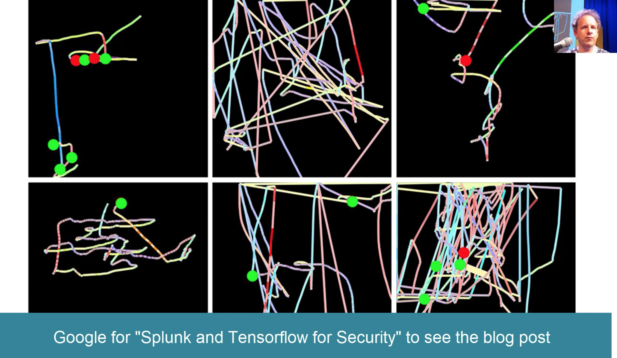
Remember earlier Jeremy mentioned that one of the fastai alumni who work at Splunk which is a NASDAQ listed big successful company created this new anti-fraud software. This is actually how he created it as part of a fastai part 1 class project.
He took the telemetry of users who had Splunk analytics installed and watched their mouse movements and he created pictures of the mouse movements. He converted speed into color and right and left clicks into splotches. He then took the exact code that we saw with an earlier version of the software and trained a CNN in the same way we saw and used that to train his fraud model. So he took something which is not a picture and he turned it into a picture and got these fantastically good results for a piece of fraud analysis software.
So it pays to think creatively. So if you are wanting to study sounds, a lot of people that study sounds do it by actually creating a spectrogram image and then sticking that into a ConvNet. So there’s a lot of cool stuff you can do with this.
So during the week, get your GPU going, try and use your first notebook, make sure that you can use lesson 1 and work through it. Then see if you can repeat the process on your dataset. Get on the forum and tell us any little success you had. Any constraints you hit, try it for an hour or two but if you get stuck, please ask. If you can successfully build a model with a new dataset, let us know! Jeremy will see us next week.
Summary
Steps of creating a world-class Image Classifier:
1. Import data
data = ImageDataBunch.from_name_re(...)
2. Build model
learn = create_cnn(...)
3. Unfreeze model
learn.unfreeze(...)
4. Find a good learning rate(s)
learn.lr_find(...)
5. To fine-tune the model train once again
learn.fit_one_cycle(...)
6. Analyze the results
ClassificationInterpretation.from_learner(...)
 Here’s a tip that can make it even nicer. For all of your code blocks, format them like this:
 Just trying to help to maintain a tidy and organized forums for everyone, like what we have done for v1 and v2 forums
 . Anyways ur notes are very helpful, thanks a lot