This is a forum wiki thread, so you all can edit this post to add/change/organize info to help make it better! To edit, click on the little pencil icon at the bottom of this post. Here’s a pic of what to look for:
<<< Wiki: Lesson 7 | Wiki: Lesson 9 >>>
Lesson resources
- Lesson video
- Course Notes from @timlee
- On Blogging by Rachel Thomas
- Universal Approximation Theorem walkthrough by Michael Neilsen
- mathematics walk-through of random initialization of matrix weights
From Forests to Nets
Random Forests Regression (RFR) is great. This model is immune to most of distributional assumptions about how we handle data. We don’t have to normalize data (which usually means taking the mean of the data and dividing by the standard deviation) to make the model work effectively. We don’t have to transform categorical/labelled data into numeric data. Also, the scale of the independent variable of a RFR doesn’t matter because a RFR makes its split decisions on where a variable is in the sort order. It furthermore doesn’t matter if variable is an outlier. Other measures that care about sort order over scale are Area Under the Curve (AUC) accuracy and Spearman Correlations. RFR is wonderfully flexible, unfussy about outlier values and capable about handling most data type situations. RFRs are hard to screw up and come with so little assumptions.
But RFR will only take you so far. You’ll place in the top 10 of a Kaggle competition but won’t win where a thousandth of accuracy matters. RFR can’t extrapolate to new data. It’s basically a very clever finding Nearest Neighbors tool; there’s a limited complexity that it can handle. An RFR works by way of means clustering. You’ll be able to solve most problems, but you’ll run into limitations with data that has a lot of cardinality in its categorical data. RFR can even run on image recognition, but it can’t handle spatial information, which ends up being important in computer vision.
Enter Neural Nets and Deep learning. Neural Nets are a class of algorithms that support the Universal Approximation Theoreom ). Basically we approximate any function with a multi-layered set of functions ( a net of functions) as long as we make the network big enough. And the derivative of this network of functions will tell us how to tweak a variable to get a closer approximation.
Mathematically, we do a matrix multiply for every layer of the neural net. Deep learning is ultimately doing a lot of linear algebra where you throw away all the negative numbers and replace the negative numbers with 0.
Practically, we’re getting multiple perspectives on a data set so we can make a decision about how to organize or classify the parts that make up the whole. For example, let’s say we have a blueberry ice cream with lime cream dessert served in a square shaped plastic cup. Our first view of the dessert is from the top (the Cartsian coordinates view on the left). Maybe, I really really hate lime cream and only want blueberry ice cream part, and from my current Cartesian view, I can’t cleanly separate out the blueberry ice cream with one knife slice.
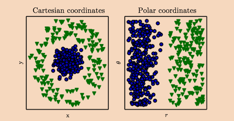
graphic source: Deep Learning (2016) by Ian Goodfellow
However, what if I can shift my perspective on the this dessert parfait? or mathematically rotate the dimension of this square dessert cup. If I rotate the dessert square cup, I can see that the blueberry ice cream part is in fact sitting on top of the lime cream (polar coordinates). I can indeed separate the blueberry ice cream from the lime with a single knife cut, because I hate lime cream soooo much (not really!)
A decision tree only has one-pass to make a decision & a random forest averages all the decisions of all its trees. A net of layered approximation functions can “look” at the same data set using different perspectives (aka different dimensions) before making a decision.
What we gain in the ability to handle complexity in data, we lose in ease of implementation. We must normalize our data and make sure that our scaling has consistent meaning across all the data. For example, we can’t normalize our training data and normalize our validation set independently. We need to negotiate that different python libraries have different ordering of its values or dimensions. We must convert all our categorical labels to numeric data. We have to learn to think in n-dimensions and to hone skills that slice into and reshape the tensor data structures.
Between Random Forests Regressors and Neural Nets, you cover most of the territory of current ML problems. You can even chain combine the two models if necessary.
Tools of the Deep Learning Trade
Nvidia GPUs is what make Deep Learning calculations possible. Nvidia’s CUDA framework, originally made for video game and movie FX rendering, is the industry standard. If you’re building a desktop box, you’ll want to spend your money buying a GPU with as much memory as you can afford. As of this writing, the 2017 Nvidia 1080ti is the best performance for the price.
Laptops:
- The GPUs in Mac don’t support CUDA.
- If you want to run Deep Learning models, you’ll need to buy a “gamer’s” laptop or MS Surface Book. You’ll want to buy one that has as much GPU memory as possible:
- You can buy a external box that could connect your GPU to a laptop via thunderbolt port, but you’d easily spend 900$ for a gpu and the box. For not that much more you could build a standalone deep learning server.
Cloud Services:
These are choices for people who don’t want to mess with buying or configuring hardware. You’ll need to be careful about turning the services off when not in use as you’ll be charged hourly or by the minute.
- The Crestle service is easiest to launch and is currently optimized for the fastai curriculum.
- AWS what industry uses and it’s worth it to spend some time learning how to manage an EC2 instance on your own. You’ll need to request the use of a GPU instance (the P2 X-large) from Amazon support, and this mayl take a few days. Then you can launch the fastas-part1v2 AMI, and then you’re all set up. Do a git pull on the fastai library to make sure your library is up to date, and then you can run your experiments or run the noteooks. You can get some AWS credits by signing up with the Github student pack.
Introduction to Language of Neural Networks.
A lot of the language of Deep Learning may seem overloaded. Deep Learning overlaps Computer Vision, Statistics, Math, and Physics, and all the fields bring their vocabulary and standard to the fields. For example, the Open Computer Vision library reads in an image’s color information as [Blue, Green, Red] and the Python Image Library reads it in as [Red, Blue, Green]. You will find yourself doing a lot of “code switching” across the overlapping academic vernaculars.
It’s OK, and recommended, to keep asking for clarification what may seem like basic vocabulary. For example, Let’s take the word “scale”. When we’re talking about an image of a cat, we can scale the image to half its current size, meaning we can make the image smaller by half. When we “scale” a single pixel value in the cat image, we’re doing something different. We’re taking the number value of the pixel (from 0 - 255), so that pixel value has an average of zero (by taking the mean of the all the pixel values) and a standard deviation of 1. In this version of scaling, we’re doing a numeric transformation where all our possible number choices are limited between 0 and 1.
There are lots of names for basically the same thing in deep learning. We’ve already seen this happen; we’ve learned that one-hot encoding or dummies encoding are basically the same thing. This will happen again when talking about deep learning’s basic data structures.
[1,2] == "vector" == "1-D array" == "rank 1 tensor"
[ [0,0],

  [1,1] ] == “matrix” == “2-D array” == “rank 2 tensor”
[

[ [0,0],

  [0,0] ],

[ [1,1],

  [1,1] ] ] == “tensor” == “3-D array” == “rank 3 tensor” (unless you’re a fussy physicist)
“negative log likelihood loss” (aka NLLLoss)== “cross-entropy”

These come in two flavors:

“binary negative log likelihood loss” is used for binary (0 or 1) decisions

“categorical cross-entropy” is used for category decisions (is the picture a cat or horse")
Practical Tensor manipulation with MNIST
The Modified National Institute of Standards and Technology database is a collection of 28x28 pixel of handwriting samples of numbers. It’s been called the “the drosophila of machine learning” or the favorite test object of machine learning researchers. Why? It’s one of the oldest image datasets for computer vision (used to solve the problem of machine reading of handwriting for the US post office), has easy to load images, and the images are easy to eyeball for correctness and difficulty. You can test your models very quickly with MNIST. For our use, the scale of the images illustrates some of the basic tenets of working with tensors, computer vision, and neural nets.
These are black & white images, but they already contain a lot of information. Every time you see a pictures, you need to know there’s a number value behind every pixel. Every image has 28 pixel rows and 28 pixel columns (28*28) and every pixel has a color value between 0-255 (the range of from white to black. If these were color images there would be three 0-255 values for each pictures representing a gradient of Red, Blue and Green), and the dataset we’ll read in has 10000 images. How do we coherently structure all this information to pass around for analysis?
This is why we need the n-dimension structures, it’s the only way to hold the different layers of information as a single entity. For example, how can we tell a computer that a number 28 means the 28th column, and not the 28th row, or not a color value in the grey range, or not picture number 28?
Introduction to PyTorch library
Pytorch functions like a GPU accelrated numpy library. PyTorch leans heavily on numpy-style syntax and Python’s object/class definition syntax. (Remember when we went over object-oriented programming?) Compared to Keras and TensorFlow, PyTorch offers a familiar interface to python programmers, more flexibility in architecting a neural net, and the ability to decide which calculations to place onto the GPU.
Let’s build a Neural Net with PyTorch
The part of the Pytorch library that does the neural net work is called torch. So we’ll import that.
import torch.nn as nn
From the PyTorch library we that there there’s class object that’s already available to us that will instantiate a model for us. We create a neural net In the same way we create a Random Forest Regressor in sklearn with RandomForestRegressor() . Sklearn’s RandomForestRegressor() has everything built-in – there are preset default parameters and settings that you tweak – and then you’re ready to run an analysis. However, PyTorch gives you a “blank” neural net container that you customize with add-ins(). The difference would be like buying car vs a car kit; with the latter you’re ordering a Toyota Prius, with PyTorch, calling nn.Sequential() is like ordering a car shell with wheels.
The module is called “Sequential” because it will run all the modules you put inside in the sequence order that you’ve placed all the interior modules.
So let’s get our kit and let’s fill it up with cool options!
your_neural_net = nn.Sequential(

  nn.Linear(28*28, 10),

  nn.LogSoftMax()

  ).cuda()
What did load into our neural net shell?
nn.Linear(28*28, 10) is module that take in an input-- here we said a defined input is (a 28x28 pixel matrix, 10-labels (our numbers 0-9) ). it’ll process these using a linear function and hold internal variables for its weight and bias (this variables are built-in to the Linear() object )
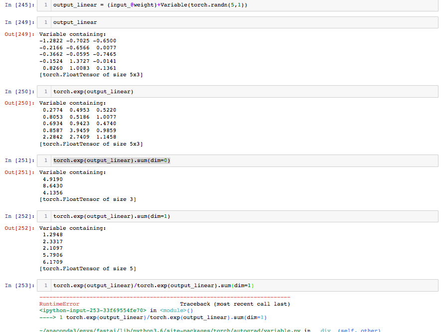
nn.LogSoftMax() is module layer that does our classification. We told our Linear() module that we’re passing in a vector of 10 classification choices or labels [0,1,2,3,4,5,6,7,8,9] . For example, after we pass one 28*28 pixel image in the MNIST through our Linear() layer, this classifying layer will decide/return the probability that the pixel image matches a label. Let’s say the softmax classifier returns [.01, .89, .01, .01, .01, .01, .01, .03, .01, .01] --> this neural net is pretty confident the image is a number “1”
(here’s a pretty good walkthrough of the math underlying the softmax layer)
.cuda() says run the whole shebang on the GPU. (aka your speed boost button)
Don’t need to calculate derivatives because the library does it for you. No one should ever need to calculate derivatives themselves…ever. As a practitioner, what you’ll need to know is why we take the derivative and the chain rule, and that’s it.
With this code, we made a 2-layer neural net comprised of 1 linear layer followed by 1 non-linear activation layer. Without any further layers, this neural net is basically a linear regression model that runs on the GPU.
Loading the image data for the neural net
The fastai library creates an object the optimizes loading image date for neural net analysis. The fastai library uses a model-data concept that wraps ups training data, validation data in a single object, and optionally test data. The ImageClassiferData also will provide batches of that data in a form ready for use by a PyTorch model.
model_data_object = ImageClassifierData.from_arrays("path/to/image/data", (x_training,y_training), (x_validation, y_validation)
ImageClassifierData is the fastai designed data object that holds the all the image data
from_array() takes in several parameters: the file path to the images,;(x_training,y_training) must be a tuple of attribute names for your training data; (x_validation, y_validation) is also tuple of attribute names for your validation data.
You can check that you data loaded properly with
x_training.shape which will output the shape of your training data, which should be (50000, 784) in the lecture demo
But what do these numbers mean?
50000 is the number of images in the training sample
784 is the flattened vector of the original image’s 28x28 pixel matrix
Training the model
.fit() is the function that trains the model with your image data. You’re “fitting” the model to your training data.
Let’s break down the parameters for this function fit(net, md , epochs=1, crit=loss, opt=opt, metrics=metrics)
net = your neural net model
md = (aka model_data object) the data being analyzed
epochs = number of times the net goes over the image, here it’s only once
crit = the loss function of your choice
opt = the optimizer of your choice : here’ we’re using the Adam optimizer with optic.Adam.(net.parameters())
metrics = the type of metrics you want to print out/ display, here we’re using with [accuracy]
Defining the Loss function: creating metrics to measure performance
We need to have a performance measure into order assess how well our net performs. If I pick up the car analogy again, we can measure how well we think our car is doing by looking at acceleration speed, miles per hour gasoline usage, engine revolutions etc. Since we’re making our own neural net model, we’ll need to pick a specific method of measuring it’s success. PyTorch has several Loss modules available.
Earlier, we measured information gain in our Random Forest Regression as Root Mean Square Error (RMSE). With Neural Nets, we’ll use negative log likelihood ( in code loss = nn.NLLoss() )
nn.NLLoss() is a our module of choice here, and it works out of the box. If you want to fiddle with its optional parameters you can check out those out in the documentation.
This loss module takes the derivative of the loss with respect to the weight matrix that we’re multiplying to figure out to figure out how to update the model. When the output of the loss function is lower, your model is doing better.
under the hood of NLLoss() is basically a function that works similarly to:
y = actual_data_point

p = prediction

def binary_loss(y, p):

    return np.mean( -(y * np.log( p ) + (1-y)*np.log(1-p)) )
A challenge would be to take this binary loss entropy function and scale it to assess categorical cross-entropy.
The role the loss function plays in the neural net would be to measure the loss and then the neural net will update the weights to reduce the loss. If your neural net is working and is “learning” you would see the loss metric go down.
Making Predictions
The neural net will make predictions using the predict() function:
pred = predict(net, md.val_dl)
net = your trained model after you called .fit() on it.
md.val_dl = the validation data being stored as an attribute within your model_data object
If we check shape of pred with pred.shape, the output will look like
(10000, 10) where we’re validating on 10k images, and 10 labels.
Here’s a reminder how the index positions correlates with the axis position
pred[0] == axis 0 == number of images

pred[1] == axis 1 == number of  possible labels for the prediction
“argmax” is an important mathmatical concept that doesn’t seem to be taught anywhere but turns out to be important in practical machine learning.
Just what isargmax()? it’s a way to convert our probabilities that LogSoftmax() returned back into predictions.
pred.argmax((axis=1)[:5]

output: array([3,8,6,9,6])
What happened here? We applied argmax() on the axis=1 of the our predicted values on images in our validation data. And we’ll peak at the first five predictions out of our 10k images. Our trained model thinks : md.val_dl[0] is a “3”, md.val_dl[1] is a “8”, md.val_dl[2] is a “6”, and so on
Checking our model’s accuracy
We get our accuracy score np.mean(pred — y_validation of the model by taking the mean of the difference between the prediction and the validation labels.
And since we’re working with image data, we can eyeball the accuracy by displaying the images alongside it’s predicted label in the notebook with
plots(x_imgs[:8], titles=preds[:8]
Here, we’re comparing the first 8 images with the first 8 label predictions. Our model got 2 out 8 images wrong, but that’s not a bad start. We’re only using a single-layer neural net which is basically logistic regression and you can get comparable results with sklearn’s model. However, our PyTorch version runs faster because it’s running on the GPU.
We haven’t built a deep neural net, but we’ve made a pretty good start. And we still have lots of room to improve.
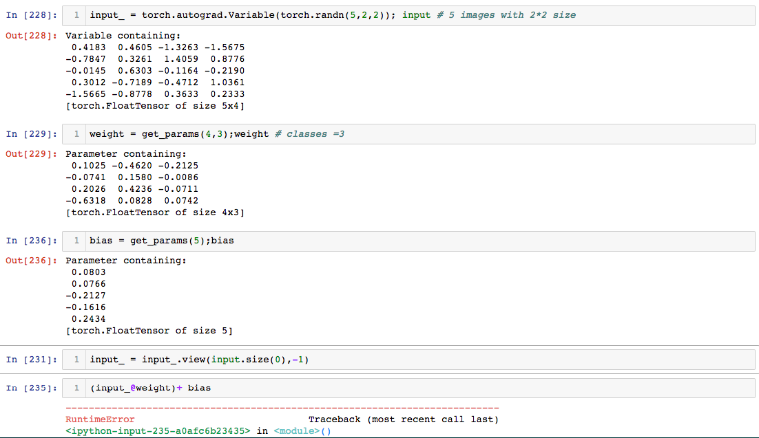
Let’s build Logistic Regression from scratch
Building Logistic Regression from scratch in PyTorch lets us explore what’s “under the hood” when we call the Linear() module.
Homework / Experiments
- try and write a first blog
- get comfortable working with tensors: reshape, flatten or unflatten ranks, slice into tensors or reverse matrices.
- play with the
torch.randn()to create random tensors andtorch.matmult()to do matrix multiplication - build out your own binary loss function using an
if-statementand then scale it out to work as a categorical cross-entropy loss function - write your own softmax function
- work through one of the PyTorch tutorials
- generally become more familiar with the PyTorch library