Wiki / Lesson Thread: Lesson 7

This is a forum wiki thread, so you all can edit this post to add/change/organize info to help make it better! To edit, click on the little pencil icon at the bottom of this post. Here’s a pic of what to look for:

<<< Wiki: Lesson 6Wiki: Lesson 8 >>>

Lesson resources


Finishing up what we know about Random Forests

When to leave the Random Forests

Just posted the lesson video.

Question - When we build an ensemble of trees, how does the code know which columns to split on for a particular tree?
For example, tree1 would split on ‘YearMade’ followed by ‘MachineHoursCurrentMeter’,
while tree2 could split on ‘MachineHoursCurrentMeter’ followed by ‘Coupler_System’.

Asmita, did you ever get an answer for this?

Take a look at the code we wrote in class together, and re-watch the previous 2 lessons before that, where we learnt the steps, and then implemented the code from scratch to do them. Then come back here and summarize as best as you can what we covered in the lessons about this and how the code we wrote works, and then we can help fill in any gaps or make any corrections as needed. How does that sound?..

1 Like

thanks Jeremy!
@daschumacher, yes I did understand this part. Forgot to mention it here.
So if we look at the TreeEnsemble class in the code, we are randomly shuffling the order to rows and columns for each tree.
This ensures that each tree would split on columns in a different order.

def create_tree(self):
idxs= np.random.permutation(len(self.y))[:self.sample_sz]
return DecisionTree(self.x.iloc[idxs], self.y[idxs],
idxs=np.array(range(self.sample_sz)), min_leaf=self.min_leaf)

1 Like

@jeremy really liked the way distribution concepts were applied to estimate certain aspects of model accuracy confidence intervals etc. Can u point to any good resource that explains the concepts of statistical distributions in a more practical way like this so that we can apply in various scenarios rather than just theory and equations

Question: in the TreeEnsemble for RF we use mean of tree predictions. Can we use logistic regression/simple single-layer neural net to get better weights between the trees? Any downsides (beside increased potential for overfitting and additional hyper-parameters tuning)?

In this post we’ll delve into the math behind the code for std_agg(), the function that @jeremy created to compute the standard deviation of a one-dimensional data vector, discussed in the Lesson #7 video, starting at the 45:32 point.

In the std_agg() function, @jeremy employs the following expression for mean squared deviation:

sum((x - <x>)**2)/N = <x**2> - <x>**2

If you’re curious about this basic result from statistics, read on!

The standard deviation is a measure of the spread or dispersion in a set of real values. Mathematically, it is computed as the root mean squared deviation. Don’t worry if you are unfamiliar with these terms; we’ll discuss them below.

The definition of the standard deviation of a vector of values x is

std(x) = sqrt( sum( (x - <x>)**2 )/N )

In this formula,

  • N is the number of samples (x values), and angle brackets <> around a vector x denotes the expectation value, or mean of x: <x> = sum(x)/N.

  • x - <x> is called the deviation of a sample x from the mean.

  • for simplicity, we’ve used N instead of the usual N - 1 in the denominator, which is fine as long as N is large.

Let’s expand the quadratic squared deviation inside the sum in the preceding equation:

(x - <x>)**2 = x**2 - 2*x*<x> + <x>**2.

Summing the squared deviations over the samples and dividing by N.gives the mean squared deviation:

sum((x - <x>)**2)/N = sum( x**2)/N - 2*sum(x*<x>)/N + sum(<x>**2)/N

Let’s examine the right hand side of the preceding equation:

  • The first term is the mean of x**2, which is by definition the expectation value <x**2>

  • In the second term, sum(x*<x>)/N is the same as <x>*sum(x)/N, since <x> is a constant factor and can be taken outside the sum.

  • But look! sum(x)/N is the mean of x which is by definition equal to <x>, the expectation value of x. Therefore sum(x*<x>)/N= <x>*sum(x)/N = <x>*<x> = <x>**2. So the second term becomes -2*<x>**2

  • The third term is just <x>**2, a constant: summing over the samples means just multiplying by N.

Adding together the three terms, we find that the mean squared deviation is

sum((x - <x>)**2)/N = <x**2> - 2<x>**2 + <x>**2 = <x**2> - <x>**2

Note that this is the mean of the squares minus the square of the mean

By its definition, the standard deviation is the root mean squared deviation, so now we just need to take the square root:

std(x) = sqrt(sum((x - <x>)**2)/N) = sqrt(<x**2> - <x>**2)

In @jeremy’s notation, cnt is the number of samples N,

s1 is the sum of the sample values x, so <x> = s1/N = s1/cnt,

s2 is the sum of squares of sample values, so <x**2> = s2/N

The formula for standard deviation becomes

std(x) = sqrt( s2/cnt - (s1/cnt)**2 )

And thus @jeremy’s function definition is

def std_agg(cnt,s1,s2): return math.sqrt( (s2/cnt) - (s1/cnt)**2 )

This formula speeds the computation of the standard deviation: its inputs are the sum of the data, and the sum of the squares of the data, both of which are O(N).

5 Likes

Hi everyone,

I believe no one has mentioned this yet (if they have and I didn’t see it, I’m sorry):

There is a minor error in the lecture at 12:40. The standard deviation of the Bernoulli distribution is actually sqrt(p(1-p)), not p(1-p).

2 Likes

Hi all. If you are running this and want to use V1 of the fastai library, I have converted over most the code to be V1 friendly. The structure is largely the same, with just a few technical tweaks on how stuff is passed around. It is actually a lot easier to convert over to V1 than the random forest part was, where functions were completely gone.

My gist is here: https://gist.github.com/mnye/339d7dfe08c881648d135e641b02ee09
It’s largely based off https://docs.fast.ai/vision.html + looking at the code on github.

This just covers the vision / lesson4 portion. Lesson 5 is next on the list! Hope it helps.

1 Like

Really love this! Thanks a lot!!!

ThreeEnsemble randomly pick different set of data for each tree, but does not shuffle the order to columns, so each tree would split on a column that create smaller standard deviation with respect to original standard deviation of the parent node.

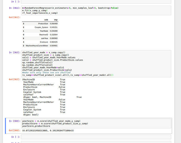
Question: Was trying to implement my own feature importance, i noticed something with sk-learn’s feature importance.

.
In the SS attached, ProductSize has higher importance than YearMade, but when I shuffle these two columns, shuffling YearMade seems to drop the score lower than that of ProductSize, which means YearMade is more important than ProductSize! Does sk-learn compute feature_importances_ in a different way, or am i doing something wrong here? Thanks!

Hi, Jeremy.

Is there a place where we can check the code you asked to do?
Thanks)

def find_better_split(self, var_idx):
x,y = self.x.values[self.idxs,var_idx], self.y[self.idxs]

for i in range(self.n):
    lhs = x<=x[i]
    rhs = x>x[i]
    if rhs.sum()<self.min_leaf or lhs.sum()<self.min_leaf: continue
    lhs_std = y[lhs].std()
    rhs_std = y[rhs].std()
    curr_score = lhs_std*lhs.sum() + rhs_std*rhs.sum()
    if curr_score<self.score: 
        self.var_idx,self.score,self.split = var_idx,curr_score,x[i]

I have a quick question here. Since the standard deviation is itself a mean of squared distances from mean. Should the score computation be
curr_score = lhs_std + rhs_std instead of
curr_score = lhs_std*lhs.sum() + rhs_std*rhs.sum()
Kindly advise. Thanks.

# First you take copy the .values
vals1 =   S.yearMade.values

# Suffle vals1

# Then put it back, but not on 
#  S.yearMade.values = vals1

# You do on the dataframe column
S.yearMade = vals1

Maybe that is altering your results.

@jeremy

I just watched your video. I wanted to share why I think your version of Random Forest did slightly better than sklearn’s. In your implementation, you tried to use every number in the column as a split point, but I’m fairly confident sklearn does two things differently:

  1. sklearn uses the medians between points in addition to (or perhaps instead of) the actual points.
  2. sklearn might also have a different (random) way of breaking ties between two columns that produce the same information gain.

To show this, download the folder at this link:
https://drive.google.com/drive/folders/1DSwQviE2vl6oOUARshT8onPompMCogL_?usp=sharing
I’ve put a small dataset and a jupyter notebook that trains a forest on the dataset so you can see why this may be the case. You can also refer to the images I’ve put in the folder. Both are visualizations of forests made using the same parameters (randomness turned off) and the same dataset, but gave different trees. This led me to believe sklearn might break ties differently, which could explain the difference.

npq should be the variance of a binomial distribution

Hi jerrmy,

Why paperspace is not supported by fastai in the new 2019 deep learning course?
I wanted to know the template available in the paperspace is updated or not?