Using use_clr_beta and new plotting tools

I’ve written a few things for the fastai library while working on my project around Leslie Smith’s last article and I wanted to share them with you.

use_clr_beta : This is the implementation of Leslie Smith’s 1cycle policy as detailed here. He recommends to use a cycle like this one:
art5_lr_schedule
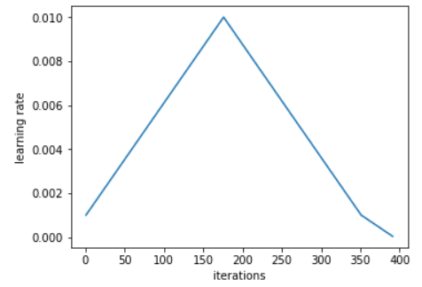
for the learning rates during the training: equal time growing and descending, and a bit of space left to get the learning rate really slow.
When used in fit, the value at the top (here 0.01) is the learning rate you pass. It should be the learning rate you pick with lr_find() and you can even choose values closer to the the minimum of the curve for super-convergence.
use_clr_beta takes two basic arguments, four if you want to add cyclical momentums. The first one is the ratio between the initial learning rate and the maximum one (typically 10 or 20). The second one is the percentage of the cycle you want to spend on the last part (on the picture 350 to 400), 10 seems to be a good pick once again.

Leslie Smith recommends to use cyclical momentums to complete this, which looks like this:


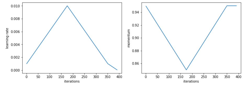
To use it, just pass two more arguments to use_clr_beta, the maximum value of momentum and the minimal value. All in all, a typical use would be:

use_clr_beta = (10,10,0.95,0.85)

I haven’t fully tested it with Adam yet, it’s originally intended for SGD with momentum.

plots: At the end of a very long cycle, if you want to do a plot with your validation accuracy or your metrics, you can find those in the variable learn.sched.val_losses and learn.sched.rec_metrics. They’re recorded at the end of each epoch.

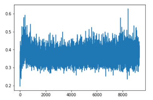
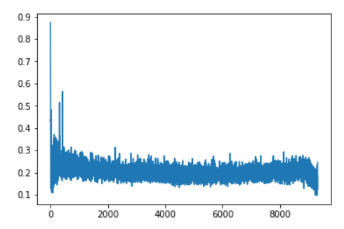
lr_find2(): As I was trying to replicate some of the curves of Leslie Smith, I wrote a second version of lr_find(). It does roughly the same thing with two differences:

  • it computes the validation loss and the metrics at the end of each batch, on the next batch of the validation set (so it’ll be a bit slower). At the end, you can find those in learn.sched.val_losses and learn.sched.rec_metrics once again.
  • it doesn’t do a full batch but rather a certain number of iterations (100 by default). That’s enough for a plot, and it’ll loop again at the beginning of the training data if your dataset is small, or do less than a full batch if your dataset is large.

On top of the arguments of lr_find(), it has num_it (default 100), the number of iterations you want, and stop_dv (default True) that you can set to False if you don’t want the process to stop when the loss starts to go wild.

Once you’ve completed a learn.lr_find2(), you can plot the results with learn.sched.plot(), and on top of having the (training) loss vs the learning rate, you’ll also get the validation loss and the metrics. By default, it smoothes the data with a mean average (like fastai does for the training losses) but you can turn it down with smoothed=False.

Hope you find any of those functions helpful!

34 Likes

Thanks for the wonderful description (and the code)!

You’re so welcome. It would never happened without your teaching and all your tips (can’t believe I had never tried the python debugger before lesson 8!) so I should be the one to thank you.

7 Likes

Since it’s all fairly new, I wanted to use this thread to ask other fastai users who used the 1cycle policy to share the situations where it worked and where it didn’t (or did less), so that we all get a better understanding on when to use it.

In my (short) experience this works miracles when trying to make a model learn from scratch (as Jeremy proved in last lesson) but less so when you work with a pretrained model you want to fine-tune to a specific situation. In particular, I didn’t find good results (not as good as Adam with use_clr for instance) when trying to first train the added layer with a 1cycle, then unfreeze and train the whole network with another (using differential learning rates) but perhaps I did it wrong. What gave me better result was to train quickly the added layer then do a long 1cycle for the unfrozen network.

In general, one longer cycle always gives better results than doing two shorter ones in a row.

It is a disaster with Adam: the training diverges once out of two, and you can’t use as high learning rates. I may have an explanation for that. The general idea of Leslie’s paper is that during the 1cycle training, we’ll get in a flatter area of the loss function and high learning rates will allow us to travel through it quickly. Flatter means lower gradients, and in Adam with divide each parameter by the moving average of the gradients squared. So high learning rate divided by a little something means explosion.

To support this, I’ve recorded the mean of all the absolute values of the gradients in my training of a resnet56 over cifar10, one with a 1cycle and one at constant learning rate.

This is during the constant training:
losses_cst

This is with the 1cycle:
error_clr

There are a few spikes at the beginning but we indeed end up fairly quickly in a reasonably flat area, which seems to be very wide in the sense that the gradients don’t spike as high as with a constant LR. The slope at the end corresponds to the part where we decrease the learning rate further, which means we get closer to a minimum of the loss function (but it’s also the part where we overfit more).

That’s for my feedback at this stage, looking forward to reading other’s experience!

6 Likes

That’s an interesting insight @sgugger . Are you avoiding the weight decay issue with adam? You should use_wd_schedule I guess.

BTW you might be interested in trying our LARS: https://arxiv.org/pdf/1708.03888.pdf . It should be pretty easy to implement in fastai - just add a callback at the start of each epoch to set discriminative learning rates. You could calculate the rates just on the validation set, to avoid introducing overhead. I don’t know if this would work for transfer learning - but for training from scratch I wonder if it would help achieve super convergence more often? (I still haven’t gotten it working on imagenet, so that’s the big goal now!)

2 Likes

Yeah I’ve tried Adam with or without weight decay (with use_wd_schedule), with or without lowering the beta2, making the beta1 follow the same pattern as the momentum or not, but nothing worked properly.

LARS sounds interesting, and it’s definitely worth a try. I’m having trouble getting some good results on wikitext-2 so superconverence might not be as universal as we thought.

So I’ve looked at the paper and implemented their version (where they change the layer parameter at each batch). Calculating the learning rates on the validation set seemed hard to me since we don’t compute the gradients for this.

It turns out is super easy to implement in pytorch since the basic SGD optimizer already updates the parameters one group (so one weight matrix or one bias vector) at a time, which the p in group[‘params’] in their step function, so we can calculate the adaptive learning rate there. I just copied/pasted the source code and added the relevant bit from their algorithm. It’s in this gist for anyone who wants to try, then you just have to type

learn.opt_fn = LARS

before running the usual LR Finder and fit.

Edit: There was a little bug in my initial code and this doesn’t work at all with 1cycle.

3 Likes

@sgugger that’s cool. Think there might be a bug?:

                d_pn = d_p.norm()#new
                if weight_decay != 0:
                    d_p.add_(weight_decay, p.data)
                    dpn.add_(weight_decay, p.data.norm())#new

That last dpn should be d_pn perhaps?

Yes, forgot to update my gist after correcting it in my notebook, thanks for pointing it out!

I kept the eta since they had one in the paper, but I wonder what’s its use since we update with lr * rho (so lr * eta * the fraction for this layer) at the end, which means we have two multiplicative factors: our initial learning rate and this eta (default 0.001). That allows them to make the reader believe they use very high learning rates (up until 32) but everything being multiplied by this 0.001, in the end, it’s not really high.

1 Like

The training diverges once out of two, and you can’t use as high learning rates. I may have an explanation for that. The general idea of Leslie’s paper is that during the 1cycle training, we’ll get in a flatter area of the loss function and high learning rates will allow us to travel through it quickly. Flatter means lower gradients.

I got a training divergence the first time I tried it. I was using the LM notebook with Adam, basically exactly as in git, but trying use_clr_beta. Because I’m training something odd (sentencepiece model of misc source code), I’ve kept the learning rates low, in the 1e-4 to 1e-3 range, so this failed with a lr of 5e-4. I had just run an lr_find that was good until 3e-3.

I started playing with this a bit (thx for your help @sgugger on understanding some of the finer points :slight_smile: ) and hope to give it a bit more time over the next couple of days.

The big news is that Leslie Smith published code for his last paper on github a couple of days ago:

It is caffe code and unfortunately is quite incomplete, but has some info that might be useful for reproducing results / experimentation. For example, it has the 3 layer model which I am planning on implementing and experimenting with.

I wanted to use this thread to ask other fastai users who used the 1cycle policy to share the situations where it worked and where it didn’t (or did less), so that we all get a better understanding on when to use it. In my (short) experience this works miracles when trying to make a model learn from scratch (as Jeremy proved in last lesson) but less so when you work with a pretrained model you want to fine-tune to a specific situation. In particular, I didn’t find good results (not as good as Adam with use_clr for instance) when trying to first train the added layer with a 1cycle, then unfreeze and train the whole network with another (using differential learning rates) but perhaps I did it wrong. What gave me better result was to train quickly the added layer then do a long 1cycle for the unfrozen network.

I’ve been playing around the last week trying to use it for better results on a Kaggle comp (iMaterialist Furniture) which takes 10+ hours per run. Unfortunately, I’ve not been able to use any of these innovations to improve against basic use_clr. If anything, it has been the reverse of your experience- 1cycle helps a touch tuning the last layer when frozen but performs worse than clr when unfrozen.

1 Like

Any details about it’s performance with RNNs, GRUs and LSTMs?

Little update on this.
I have been trying for two weeks to make super-convergence work on wikitext-2 (another small subset of wikipedia already tokenized by Stephen Merity and for which there is benchmark available) and it was working a bit, but not too much (and driving me crazy!)

I’ve finally figured it out and even if I’m still not in their 65.6-68.7 range for perplexity on a normal training my best is at 74 for now (I was stuck above 100 for the longest time). Though I use 120 epochs when they use 750. The key setting that changed everything was the gradient clipping. I had dismissed it at first but it turns out that in RNNs, it lets you get to really high learning rate (my best score is with a learning rate of 50 max!) without exploding.

I don’t know if it generalizes to CV or if it’s specific to RNNs, I just ran one experiment on cifar10 where adding gradient clipping gave me a slightly better result at the end (92.7% accuracy instead of 92.2% without, but it could just be random).

The fact it doesn’t get in the way of super-convergence is aligned with the idea I expressed in a previous post: in that period with very high learning rates, we are in an area of the loss function which is rather flat, with low gradients, so clipping doesn’t change a thing.

I’ll prepare a notebook with my best experiments but I’d really like to get to the SOTA result first.

4 Likes

Looks like I picked it! :smiley:

3 Likes

Not sure if I was clear: you need to keep it (0.25 like in Stephen Merity’s paper seems to be the best value from my experiments) not remove it.

2 Likes

Hi Jeremy / sgugger,

The AWD-LSTM repo contains the gradient clipping (https://github.com/salesforce/awd-lstm-lm/blob/master/main.py#L208) whereas I couldn’t find this enabled in the lm_rnn.py in fastai. Could you give me a hint on where do I look for it?

You just have to write learner.clip = your_clip_value and it’s done.

1 Like

Ah. It goes in as a part of **kwargs. Didn’t notice that. Thank you. Let me go back and try using this on my LM.

Hi @sgugger & Jeremy,

I added the gradient clipping in my LM and it has straight away given 2% accuracy improvement. There’s almost a 3% improvement in the downstream classifier.

Now, I’d like to do some more experiments to keep pushing these accuracies further. Although before that, I have a bunch of TODOs to finish up. Here is my repo: https://github.com/binga/fastai_notes/tree/master/experiments/notebooks/lang_models.

Ok, I just realised I’ve to host the stoi dictionary for others to reuse my weights. Doing it right away.

1 Like