I have done a test run of Lesson 2 , using images of eczema patients ( I am trying to create an eczema classifier .
The below are my results of the Lr_fit_one_cycle .
Total time: 00:15
epoch
train_loss
valid_loss
error_rate
time
0
10.023257
462.080811
0.781250
00:07
1
9.761022
45.259087
0.867188
00:07
I feel my error is just too high .
What can i do to improve it ?
Nothing really new, just trained the second lesson notebook on my own dataset and put it on the web. And now the algorithm will allow you to decide if a picture is of Superman or just a random journalist. I had a good time making it, that makes me excited for what’s next !
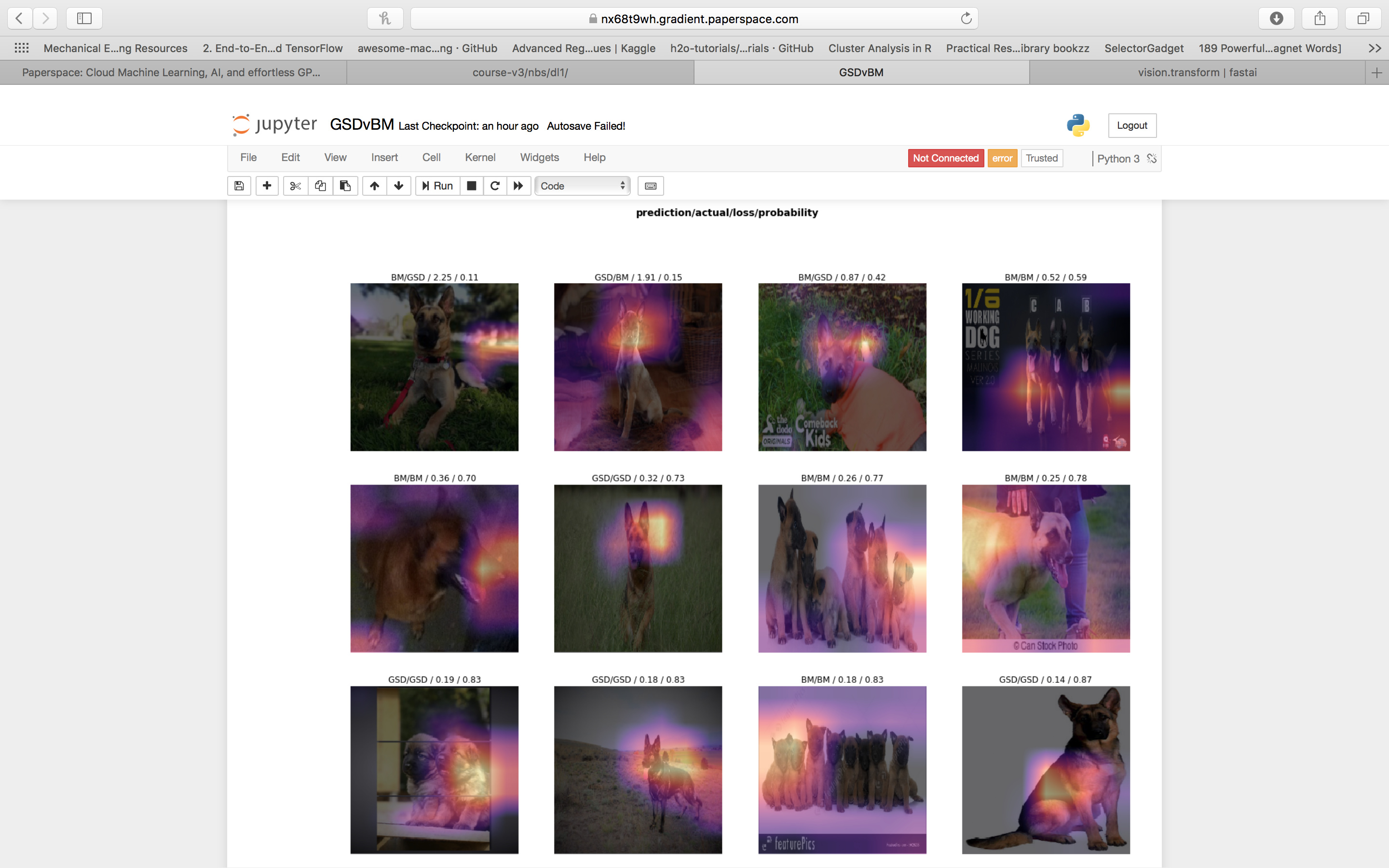
Hi all, finished watching the first lesson last week. Made a few trial projects so far. This is my German Shepherd Dog (GSD) and Belgian Malinois (BM) image recognition project. Many people find these two breeds visually similar. While I was going through the downloaded images off Google Images, I couldn’t tell the difference between the two sometimes (and I own a GSD).
This ended up achieving a 98.3% accuracy on a dataset size of 616 GSD photographs and 227 BM photographs, using a 80/20 train/valid split. I believe my results would have been similar using even less images, and I will try with a 50/50 train/valid split to find out if this hypothesis is correct.
The whole project took about 30min in total.
20min for downloading images and manually deleting unusable images / incorrectly labelled images
5min to upload data to Paperspace Gradient
5min of trialling with ResNet 34 and ResNet50.
Here is a screenshot and some notes.
Here we can see the model generally look at faces/snouts and coat colours.
Note: Out of the 168 validation images only 3 were incorrectly classified
See for yourself the similarities between the two breeds.
This is the ResNet50 model after 4 frozen epochs and 8 unfrozen epochs, which is where I stopped as the train_loss went below the valid_loss and the valid_loss stopped decreasing. The error went down to 4.16% after the first stage and 1.79% after the second stage.
I added cutout as an extra transformation which I have found in other projects to help increase accuracy when using multiple epochs to stop from overfitting.
The images were compressed to 65kb size before uploading to Paperspace Gradient
These results are better than I was expecting, but not too surprising given the results of the Cats and Dogs model shown in lesson 1.
If you have any questions or remarks, please go ahead.
One other catch with this contest is the way in which you create your validation set. The dataset is made up of slides that are taken from larger composite images that have been split into smaller 96x96 images. The test set for the competition was created by withholding a set of the larger composite images (not just randomly selecting some of the smaller images). This is an important distinction because it means that the test set consists of images that come from slides your model has never seen before, and in general that means your model will do worse on them.
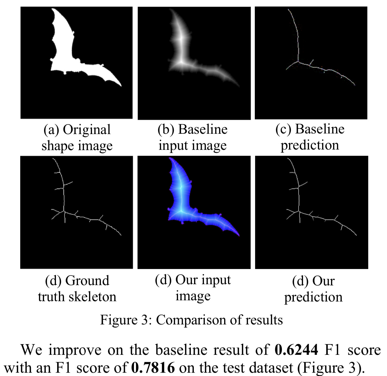
I recently competed in a CVPR 2019 Workshop challenge, segmenting skeletons from 2 dimensional binary shapes. Using an image distance transform from a 2007 paper combined with “out of the box” fast.ai U-Nets, I managed 1st and 2nd places respectively in 2 of the 3 challenge tracks. Thanks to fast.ai for the tools to compete in professional computer vision conference challenges! 14 months ago I’d never done any ML/DL/python or maths beyond high school. Awesome fast.ai.
It was interesting to participate in an academic challenge where a paper also had to be submitted. In my non-ML/DL/DS day job the pursuit is to combine cheap, supportable, proven, flexible building blocks most effectively. Isn’t that the goal in most jobs? But in paper review terms that is known as “reject - no significant novelty is introduced”. No wonder when I’m looking for a solution I avoid the deluge of dubious academic papers but instead turn to blog/forum posts of practical implementations and spend my time trying to understand the dataset, not implement last week’s networks.
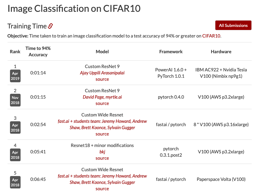
I set a new DAWNBench record for CIFAR10 training time! It’s only about one-second slower than David Page’s submission (and used the exact same code), but I still found it pretty satisfying. The only difference was the hardware.
I understand that one second means virtually nothing in practice, but I’m guessing that by using PowerAI and the AC922 chip, the percentage improvement might become more significant with larger models and datasets.
Though I haven’t had any formal CS education nor have I read about parallel processing in depth, so I’m not sure how this would scale. Can someone with more experience comment?
Hi all, would love to have feedback on this project/blog post. Not directly related to Part 1 of 2019 class, but it uses fastai v1 so hopefully appropriate to post here. The (custom, had to have fun creating a convnet called ZipNet) convnet didn’t perform as well as lgbm, curious if anyone had feedback on improvements. Thanks!
Hi @JoshVarty thanks for your reply and that was a good insight, never would have thought to have done that. After going through some of the Kaggle discussions it seems like there are some specific pre-processing being done to the images which some of the top submissions went through. I’ll try and re-compose my validation set in this way and see the difference that makes. That link in your post (and also your post : ) to the Kaggle solution was useful.
For Lesson 3 I made a segmentation model using the MultiMNIST dataset !
Available here : http://thomasdargent.com/projects/fastai2/
An easy project overall. The preprocessing steps were indeed the “hardest”.
Sure. Whenever faced with a single channel input and able to use pre-trained models, see if you can feed in extra pre-processed data alongside it. Thats generally my approach to all challenges - spend time getting the input data sorted out over making a cleverer network.
I fed in the simple Euclidean distance transform- where pixel intensities are mapped as the Euclidian distance from the pixel being evaluated to the closest border pixel.
I also fed in the “isotropic diffusion of the gradient vector field of the euclidean distance transform” described here. What a mouthful! The effect is to cause calculated pixel intensities to fall off more rapidly away from medial axes.
I enjoyed learning about the Chamfer Distance which was being used as a metric. This basically measures contour differences point by point. I reckon this might have some legs in image segmentation especially if somehow I can create a loss function in future. Seems more intuitive than Jaccard/IOU to me.
Thanks guys for providing all these amazing resources!
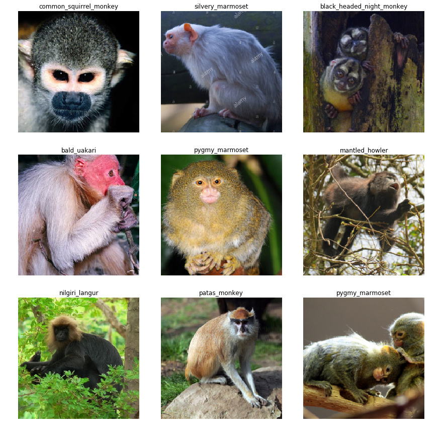
In Lesson 1 I struggled a bit with pre-processing the dataset and getting to grips with the API’s though finally got the monkey classifier working. I changed all the label directories to the monkey names and compressed and uploaded the file to google drive.
Using the code in Lesson 1 nb the accuracy was 96.8% and after unfreezing the layers and re-training the accuracy increased to 97.5%. The best entry on Kaggle achieved 98%+ using resnet34.