I’ll take a look and let you know.
I did a small experiment that suggests as networks get deeper we should train them multiple times using different initialisation parameters and use a voting scheme for inference. Below is my rational. Interested in peoples thoughts.
In the previous lessons we learnt that parameter initialisation is very important. However, Kaiming initialisation is still derived from random numbers. Therefore, we should not assume we get a good starting position when we train a network. If we just make one attempt we could get unlucky. If we try multiple attempts it reduces our chances of starting off on the wrong foot. It also means we get to explore different state space in the network because they are designed to minimise loss and that goal starts after initialisation. So if we use different starting positions and save those models for inference we increase our changes of success (because we explored a broader space that allowed the models to collectively calibrate against the data).
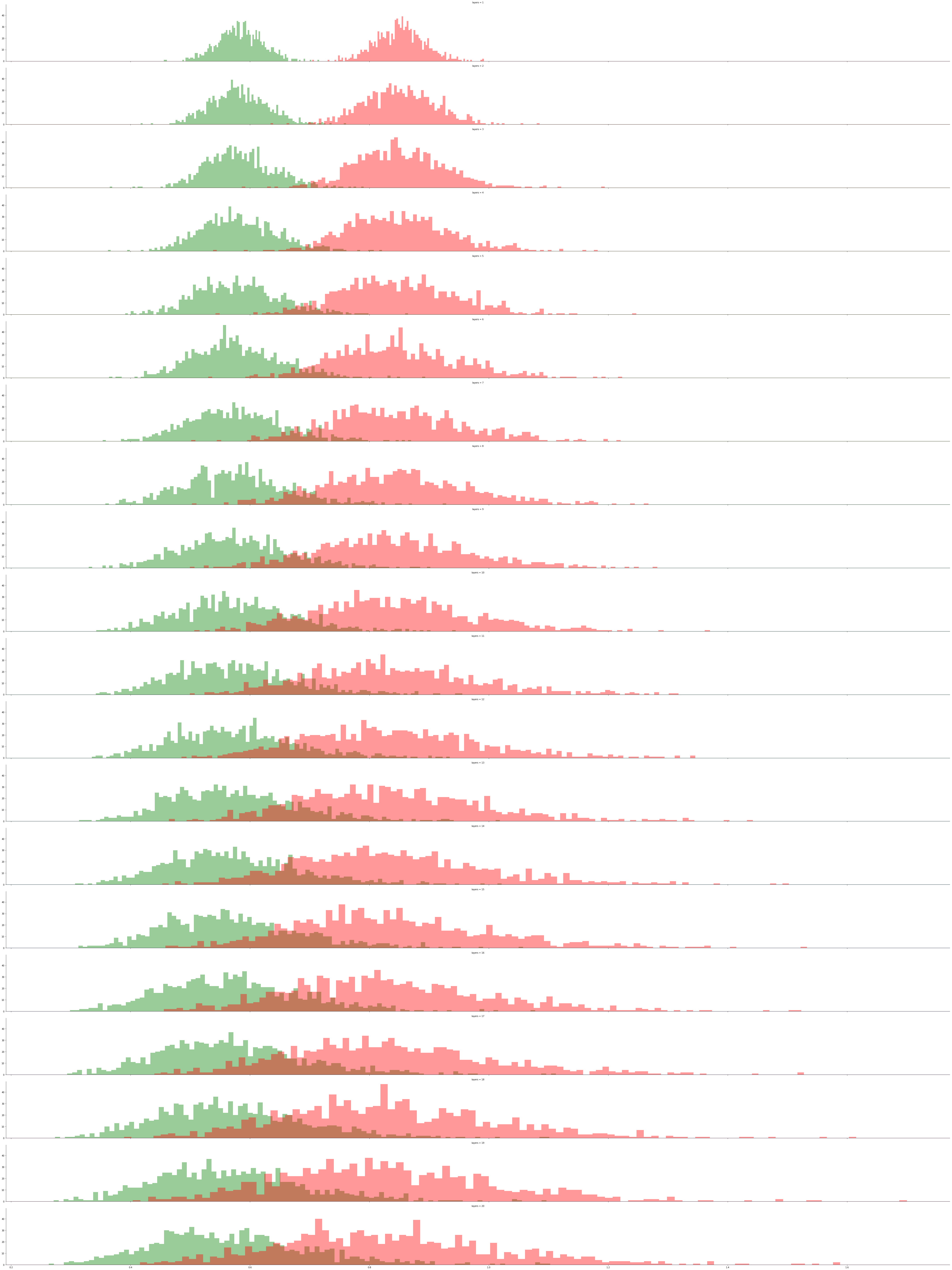
I did a small experiment to show how this might play out with Kaiming initialisation. The left and right charts (and green and red histograms) represent the means and standard deviations of the parameter space for each consecutive matrix multiplication. I simulated 1000 initialisations and performed 20 (L) consecutive matrix multiplication operations. What is interesting is the range. As L increases the range in mean and standard deviation increases which suggests we are more likely to randomly choose an unlucky initialisation as L increases. FYI I used some of @jamesd code from his great blog
def kaiming(m,h):
    return np.random.normal(size=m*h).reshape(m,h)*math.sqrt(2./m)

data = []

inputs = np.random.normal(size=512)

for i in range(1000):

    data.append([])

    x = inputs.copy()

    for j in range(20):
        a = kaiming(512, 512)
        x = np.maximum(a @ x, 0)

        data[i].append((x.mean(), x.std()))

fig, ax = plt.subplots(1, 2, figsize=(20,10))
ax[0].plot(data[:,:,0].T, '.', color='gray', alpha=0.1)
ax[0].set_title('mean')
ax[0].set_xlabel('layer')
ax[1].plot(data[:,:,1].T, '.', color='gray', alpha=0.1)
ax[1].set_title('std')
ax[1].set_xlabel('layer');

Also a histogram plot.
import seaborn as sns

layers = []
means = []
stds = []

for layer in range(20):
    mean = data[:,layer,0]
    std = data[:,layer,1]
    l_values = len(mean)
    layer += 1
    layers.extend([layer]*l_values)
    means.extend(mean)
    stds.extend(std)

df = pd.DataFrame({'layers': layers, 'means': means, 'stds': stds})

plt.figure()
g = sns.FacetGrid(df, row="layers", hue="layers", aspect=15, height=4)
g.map(sns.distplot, 'means', kde=False, bins=100, color='green')
g.map(sns.distplot, 'stds', kde=False, bins=100, color='red')
g.map(plt.axhline, y=0, lw=1, clip_on=False);
7 Likes
Interesting work.
I have a question regarding your suggestion of training multiple NN with different init and ensembling their predictions.
After having a good init (mean close to 0 and std close to one through all the layers), with kaiming or LSUV, what is the point of training the same model multiple times and ensembling their predictions?
If I want to do ensembling, wouldn’t it be much better to train NN with different architectures or hyper parameters to get more diversity (as the goal of ensembling, if I understand correctly, is to get uncorrelated errors)?
I am not sure but I think it would be a more useful use of computation?
Hi, thanks for pointing it out. Just fixed it. 
1 Like
I purposefully did not mention ensemble because that comes with its own connotations. I don’t see this replacing ensembles. I see this as another option to try and improve a models performance. I guess the proof is in the results. When I get a chance I will try it and report back.
Edit…
Having thought about it a little more it reminds me of how random forests work. A random forest produce many models (trees) and each model gets a vote. The randomness is in the features applied to each model. In the approach I’ve suggested the randomness is in each models initialisation parameters.
1 Like
This is an intriguing idea, @maral. It would be interesting to see a pilot experiment in which you implement your idea of training models with multiple initializations and demonstrate improved accuracy or reduced training time or both!
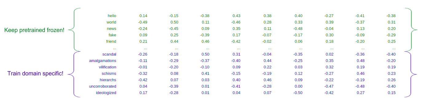
I had an interesting idea where you split the pretrained embeddings matrix in two groups: trainable and frozen. During training, you only update the indices in the vocab which were missing in the pretrained matrix and you leave the others frozen. This allows you to learn the domain specific word embeddings while leaving the more general language model components frozen.
Blog post
3 Likes
one of thing in deep learning always confuses me is to decide on proper use of weight initialization. I did lot of study on this but could not figure out any guidelines…
Created a new blog post on Semantic Image Synthesis with Spatially-Adaptive Normalization paper by Nvidia. It introduces SPADE a new normalization block for semantic image synthesis, and it achieves state of the art on various datasets for image generation.
In the blog post, I cover
- What is Semantic Image Synthesis:- Brief overview of the field.
- New things in the paper
- How to train my model?:- How Semantic Image Synthesis models work
- Then I dive into the different models that make up the SPADE project namely SPADE, SPADEResblk. Then I introduce Generator and Discriminator Models and the Encoder model for style transfer.
- Loss function is discussed in some detail and perceptual loss is also introduced with code. The original Nvidia code for loss function can be found here.
- There is a discussion on how to resize segmentation maps and how to initialize my model using He. initialization also.
- What is spectral normalization?:- When to use this normalization and a discussion on instance normalization.
2 Likes
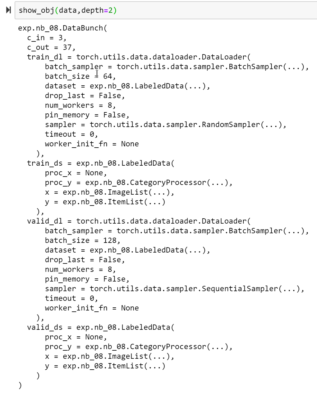
I’ve been wanting to do something like the debug callback Jeremy did for a little while now. Yesterday I came across this library ppretty and I’ve found it super helpful with printing out what each class has inside of it. This is what I did:
pip install ppretty
put this in nb_000.py:
from ppretty import ppretty

def show_obj(obj, depth=1, indent='  ', width=100, seq_length=1000,show_protected=False,
             show_private=True, show_static=True, show_properties=True, show_address=False, str_length=1000):

    print(ppretty(obj, depth=depth,indent=indent,width=width,seq_length=seq_length,
                  show_protected=show_protected,show_private=show_private,show_static=show_static,
                  show_properties=show_properties,show_address=show_address, str_length=str_length))
and put from exp.nb_000 import * in nb_00.py.
now you’ll be able to see what each class has inside it and everything you can get to from inside the class. Here are some examples:


10 Likes
Nice! FYI **kwargs would make that def much cleaner.
1 Like
I had that, but it felt like the function was kind of contradicting itself since it wasn’t showing what it could take. So I went the messy route
1 Like
Hi Everyone,
I have been a bad student during April with 0% attendance.
But I do have a little writeup from my team’s gold medal finish in the Petfinder kaggle comp to share here: Link to the writeup, Link to code.
I hope it makes up for the lack of my attendance. 
PS: I’ll graduate from college in 2 weeks and then I’ll commit full time to fastai, hoping to share at least 1 blog based on the Part 2 lectures soon. (Leaving it here so that I have no way to back down later  )
)
11 Likes
We see you… ![]()
4 Likes
Recently I was participating in CareerCon 2019. I tried to use Deep Learning models but without much success so I decided to use something very simple to get at least some result. (Interesting enough that even this simple solution helped me to get into top 7% on the private leaderboard. One more proof that overfitting could be dangerous I believe because my final position is about ~350 higher than it was on public LB so it means some other competitors lost their positions).
However, the final top-scored solution actually used a Deep Learning model. It was written in Keras, and I decided to replicate it with PyTorch in this kernel. Here is the model architecture.
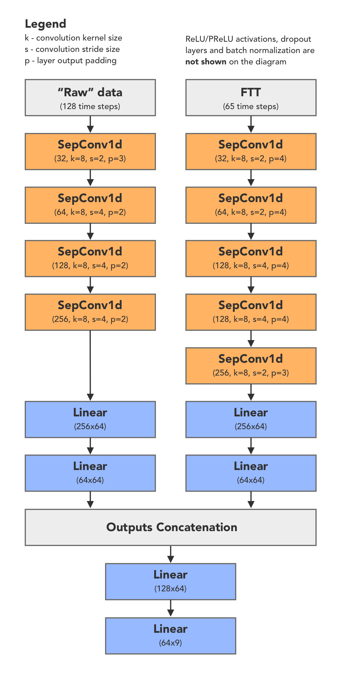
The most interesting aspect here is that I wasn’t able to get a good result with deeper models because I hadn’t really preprocessed my data correctly. I’ve used the dataset as is instead of a bit more thorough exploration. That’s why my implementations based on LSTM and 1-d convolutions worked pathetically bad, I believe. Therefore, it is not enough to just through a bunch of numbers into some network and wait it will work 
5 Likes
You also have an option to choose to be a part of metered paywall but share a “friend” link to your story on forums or in communities you would like so people who follow this link will have free access.
I think the only reason for choosing to be a part of paywall could be a better distribution of the article among Medium’s audience. Like, in this case, Medium will distribute references to your story via their channels and probably will feature your story in emails to subscribers, or something. (Though I am still not too familiar with their new system).
I tried to implement this paper: Drop an Octave: Reducing Spatial Redundancy in Convolutional Neural Networks with Octave Convolution.
The basic idea: in your convolutional blocks, allocate some channels to lower resolutions, specifically at half the height and width (image on the right).
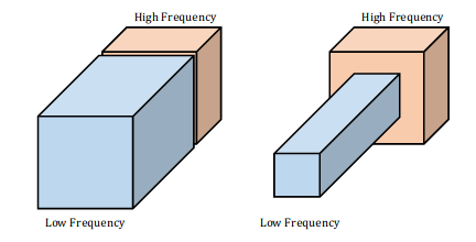
For example, if your original convolution was a 128 x 112 x 112 tensor (channel x height x width), if you split it 50-50%, it would become a 64 x 112 x 112 tensor and a 64x57x57 tensor (half the resolution).
To connect these new blocks in successive layers, you will need to upsample/pool the activations.
Why do this? First, the low resolution part of the convolution has fewer operations, making the network (in theory) faster. Second, convolutions on the low resolution block have a higher receptive field, so you may get better performance as well. (Basically, you’re splitting the work, low-res blocks learn general pattern, high-res blocks the details).
In addition, the authors tested the network on ImageNet, and beat many benchmarks.
I thought the idea was cool, so I tried out fastai’s XResnet with this new type of block. (here is the repo). However, I couldn’t get the network to beat the ‘vanilla’ XResnet performance on ImageNette or ImageWoof.
Also, my training time got a lot worse (~2-3x slower). The low-frequency convolutions have fewer computations, but maybe the upsampling/pooling adds too much overhead? I’m not quite sure. Anyway, I’ll leave the idea at that for now, and maybe rerun the experiments when the authors release their official code.
10 Likes
I figured I should keep my stories out of metered paywall.
After lesson 12, I was interested in playing around with what I learned on the to re-implement Doctor AI: Predicting Clinical Events via Recurrent Neural Networks
paper. Here’s my blog post and code.
.
9 Likes
This is a Medium post that serves as a summary of the Section 7 of Rethinking the Inception Architecture for Computer Vision paper. Section 7 basically gives us the mathematical details on label smoothing that was mentioned during Lecture 12.
1 Like