Share your work here (Part 2)

[ste (Stefano Giomo)]

TfmsManager: visually tune your transforms

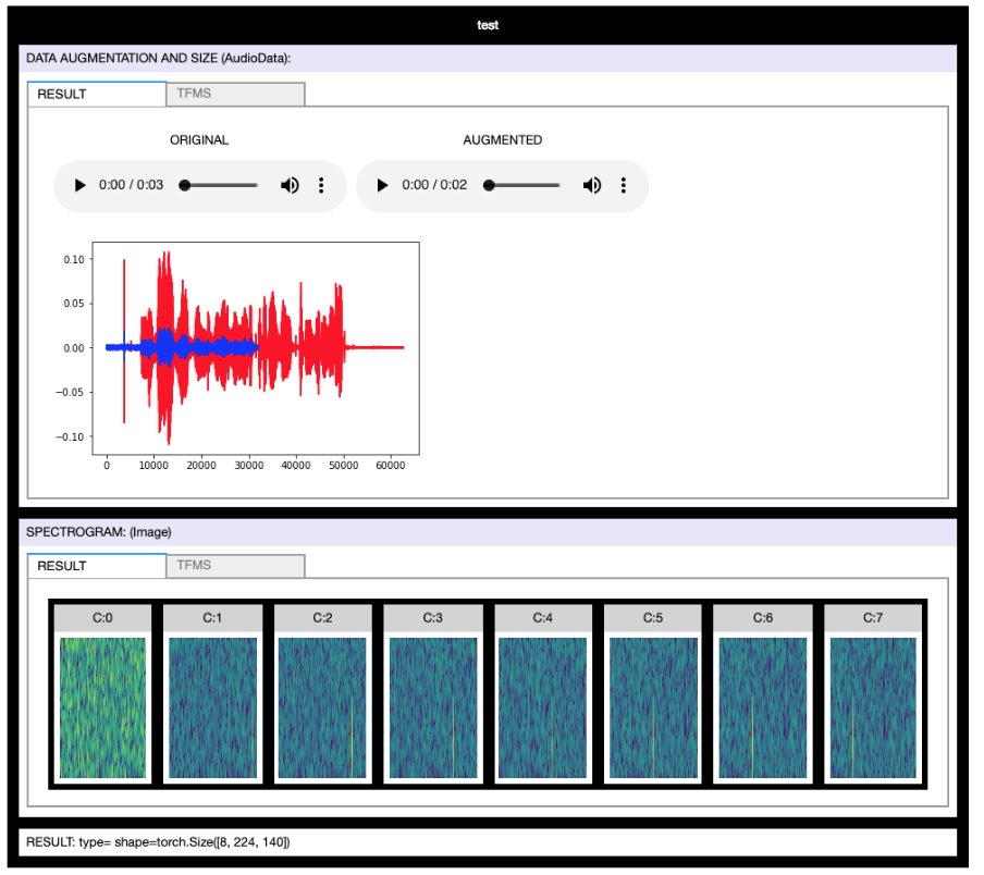
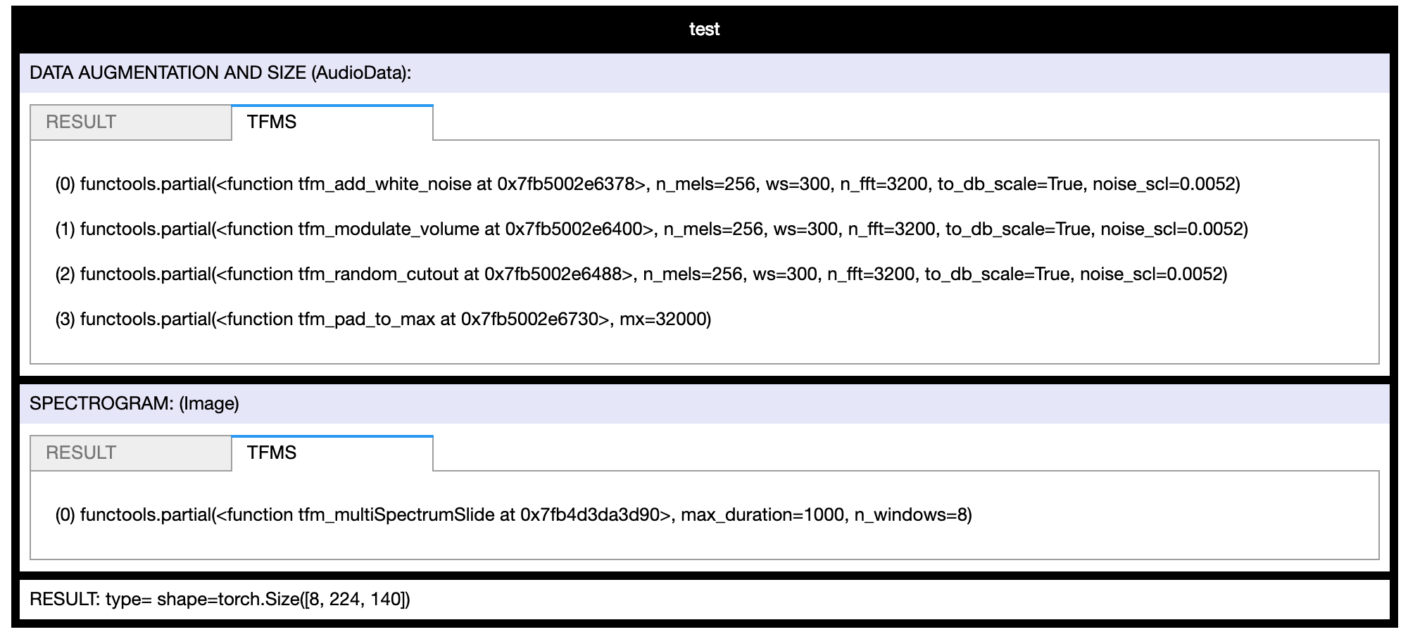
I’ve published a tool to quick visualize and tune a complex chain of data transforms (Audio & Image).

TfmsManager: Tune Your Transforms

What is that TfmsManager is an easy to use tool that helps you tune and debug complex groups and chains of transformations. It comes with a two use cases for Image and Audio transformation. IMPORTANT: you can preview your transformation before creating a “data bunch”, having only some samples (Image or Audio data). Features Preview: see the extent of modifications made by your transform. Diff: visually compare your original data with transformed one. tfms: the “TFMS” tab shows you the exa…