The refugees needs may be more urgent…
Python version
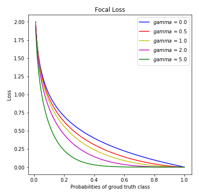
import matplotlib.pyplot as plt

fig, ax = plt.subplots(nrows=1, ncols=1, figsize = (6, 6))

pt = np.arange(0.00, 1.01, step= 0.01)
CE = -np.log10(pt)

# legend color: gamma
g = {'b': 0.0, 'r': 0.5, 'y': 1.0, 'm': 2.0, 'g': 5.0}

for i in g:
    #print(i, g[i])
    FL = (1-pt)**g[i]*CE
    ax.plot(pt, FL, c = i, label = '$gamma$ = '+str(g[i]))

ax.legend()
ax.set_xlabel('Probabilities of groud truth class')
ax.set_ylabel('Loss')
ax.set_title('Focal Loss')
12 Likes
I think there might be a problem with RandomRotate for bounding box coordinates.
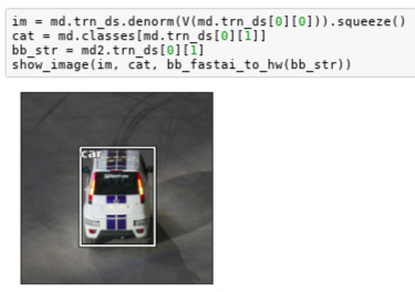
I pick an image with a very well fitted bounding box:
I then apply the RandomRotate transformation:
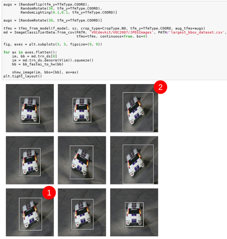
(apologies for the redefined augs in the code making it less clear to read).
The results don’t seem right. In particular, why such a big difference between 1 and 2? I remember the discussion from the class with regards to this but given how tight the bounding box is and the object being rectangular I am concerned there might be something else amiss here.
Would be very grateful if someone could please confirm if they are seeing similar behavior?
1 Like
Interesting. Maybe try putting a original target boundary box in the image itself and try augmenting that to see how the original box fits in the new one? That might make it easier to see what to look for if there is something that can be improved.
Yeah that does look odd. Would love help debugging this! ![]()
Without a doubt, that is a really, really neat way of preprocessing data ![]() I think @binga was not paranoid enough though (and neither was I when re-implementing this
I think @binga was not paranoid enough though (and neither was I when re-implementing this ![]() ). As a result, I ended up questioning my life choices and the meaning of it all we so trivially call life. Becoming a castaway and living on an island with no electricity started to seem like a very appealing lifestyle. I think anyone whoever debugged a model will understand
). As a result, I ended up questioning my life choices and the meaning of it all we so trivially call life. Becoming a castaway and living on an island with no electricity started to seem like a very appealing lifestyle. I think anyone whoever debugged a model will understand ![]()
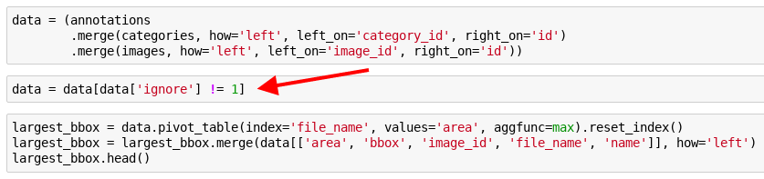
It all started with my models giving me slightly worse performance (2 - 3%) on accuracy vs the ones I worked on earlier for lesson 8. I started working back from the end of the notebook… to spare you the sappy details of this story, this is what you need to change to get results like in the lecture:
Fun fact: the datasets will still not be exactly the same as pd.merge will grab more than one entry if the area of the bb in said image is exactly the same (which it is for a single image with multiple aeroplanes).
In case anyone wonders why the difference in performance - some items, if the are not fully visible or for other reasons can be considered hard. If such, they will be marked with ignore = 1. Here is an example:
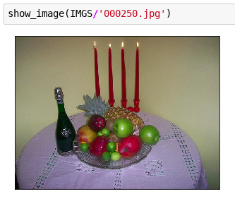
Here the biggest bb is for the… table. We can infer it is a table but just looking at the picture it might be hard to figure out what this white circular blob is. Hence, ignoring some annotations, we would go for the bottle instead (this is the biggest bb in the image with ignore == 0).
3 Likes
You have room for 1 more person?
3 Likes
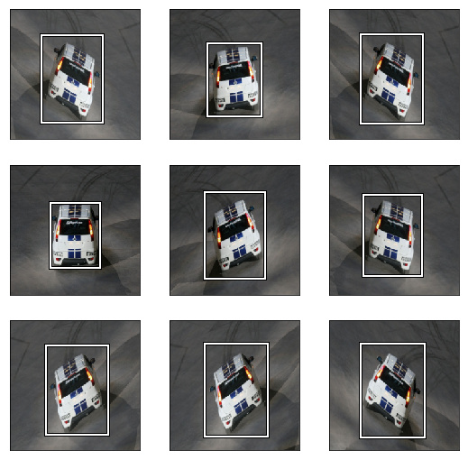
I think I found were it came from. There is a weird part of zeros appearing when we do the rotation to the box transformed in a square:

When the second picture is set to a bbox again, it tries to include this weird bit, hence making it larger.
This is obtained by redoing the steps of the RandomRotate Transform with the picture and it’s box, my code is:
rot_tfm = RandomRotate(10, tfm_y = TfmType.COORD)
rot_tfm.set_state()
rot_tfm.store.rdeg = 30
y_squared = CoordTransform.make_square(box,im)
fig,axes = plt.subplots(1,2,figsize=(12,4))
show_img(rot_tfm.do_transform(im,False), axis=axes[0])
show_img(rot_tfm.do_transform(y_squared,True), axis=axes[1])
where im contains the image of the car and box the associated bbox in a numpy array.
1 Like
The problem seems to be in the self.BORDER_REFLECT flag, it shouldn’t be used for y. I’m making a pull request on github.
It seems to work well once corrected:
6 Likes
You rock ![]() Awesome job.
Awesome job.
Your PR isn’t quite right (although I merged it since it’s better than what we have). You should check whether it’s TfmType.COORD or TfmType.CLASS and only use constant border mode in those cases. For TfmType.PIXEL we probably want reflection padding.
Oh, you’re right, I forgot about the PIXEL TfmType and in those case the pictures will have black pieces we don’t want. I’ve made another pull request correcting this.
Turns out that this also has to be eliminated or else we will be getting significantly worse results… Not sure why but seems that having a single image labeled twice as ‘aeroplane’ and thus appearing in the dataset twice throws things off. Simply deleting this row from the csv fixes this issue.
The middle two are the offending lines in the CSV:
000654.jpg,sheep
000657.jpg,aeroplane
000657.jpg,aeroplane
000671.jpg,bicycle
I wanted to share the csv files but seems the forum is not allowing them to be uploaded.
In summary, it seems that having a file labeled twice in a csv dataset, even with the same label, throws something off in the construction of the dataset and leads to examples that appear after the duplicated line to be mislabeled.
Would be great if someone using the dataset constructed from CSV (@binga’a method) is able to easily get over 80% accuracy (in the range of 82-84). If they are, then I am just hallucinating things. If they consistently get below 80%, then the problem is real.
1 Like
Thank you for the in-detail report on this Radek. I’ll check and report my findings by evening.
Perfect.
Here is a notebook with amendments to @binga’s pipeline that I think eliminates the issues.
In the repo I’ve also added the csv files:
2 Likes
So you remove the background class, because at the end of the network you don’t care about the output responsible for the background - because you don’t want to force the network to learn about this special class background
So you look only at the 20 outputs responsible for each of the classes. And if all of their sigmoid(outputs) are close to 0 - this will mean that there is background (or other unidentified object which is not between the classes).
But then why is it useful to have 20+1 classes in the first place, why we don’t use just 20?
This is a very important question.
Cropping is not recommended in object detection as it leads to loss of information about objects located at the margins.
Resizing by squishing the image seems to be the only option. The justification given for this is that the CNN is smart enough to classify even squished or deformed images.
In cases like the one u pointed out is an extreme case .
So there should be limit to what extent we should squish an image.
Just putting down my thoughts. Sorry for not answering the question.
I have a question: the last three layers whose grids are used as anchor boxes, the channel length (depth) should be equal to k*(4+c), but in the layer with 16 grids if I apply the above formula it becomes 225 but the channel length is 256. This is also the case with next two layers.
If I am not wrong, k is the different combinations of each grid cell with changes in width, Hight, zoom etc. In the 4*4 convolution layer k=189.
Hi there @chunduri , good question  …the below is my understanding:
For the SConv layers, we can sort of freely set channel length based on how many features we want to learn at each scale (I believe Jeremy mentioned he chose 256 to match the SSD paper), not based on # of predictions.
For the OutConv layers, channel length (depth) is determined by the # of predictions at each image region (grid cell). (So for a given grid cell, we can think of it as stacking that cell’s predictions one on top of the other along the channel dim.)
If we were to combine the classification task and localization task in the same tensor, you are right that this implies a channel depth of 225 (K*(4+C+1)).
However, we use separate convolutional “branches” for the two different tasks, and these are implemented as self.oconv1 and self.oconv2 within the OutConv layer class:
class OutConv(nn.Module):
    def __init__(self, k, nin, bias):
        ...
        self.oconv1 = nn.Conv2d(nin, (len(id2cat)+1)*k, 3, padding=1)
        self.oconv2 = nn.Conv2d(nin, 4*k, 3, padding=1)
(In the nb, K is set to 9, not 189: K = the number of anchor box default “types”: 3 zooms * 3 aspect ratios = 9 combinations.)
The 2nd arg passed to oconv1 and oconv2 is output channel depth:
- (C+1) * K for
oconv1, which is responsible for classification: 20+1 predictions for each of the 9 anchor box types: (20+1) * 9 = 189, hence 189 depth for o1c, o2c, and o3c. - 4 * K for
oconv2, which is responsible for localization: 4 bbox coords for each of the K anchor box types: 4 * 9 = 36, hence 36 depth for o1l, o2l, o3l.
(Note, these layers all get flattened and then concatenated into a different shape in the end. Also, the logic for channel depth applies across all grid scales.)
5 Likes
A pretrained model could handle rectangular images. However the fastai library currently doesn’t support this. A PR would be most welcome, although it would require some care in implementation. If anyone is interested in doing this, please create a new thread and at-mention me so we can discuss it.