Oh, you’re right! That’s funny because I would have expected the opposite, given the fact it’s harder to predict a category other than background with a stronger negative bias.
Loved this video, here’s a link to a spreadsheet that follows the examples in the video.
3 Likes
I was trying to attempt this and I made 2 changes.
- Removed the +1 in the oconv1 to exclude background.
- In the BCE_loss, I used all the columns -
x = pred[:,:]
instead of
x = pred[:,:-1]
for matching the dimensions.
The loss was more or less the same. Maybe I haven’t trained it well enough but there are incorrect annotation predictions.
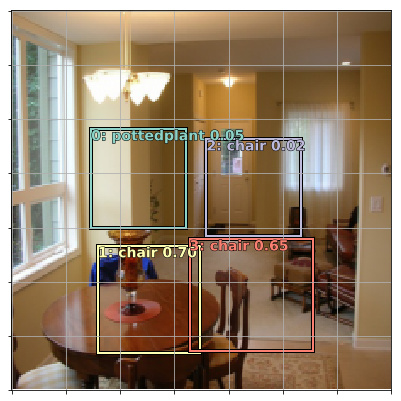
I adjusted the threshold to 0.2 and now the incorrect annotations are gone.
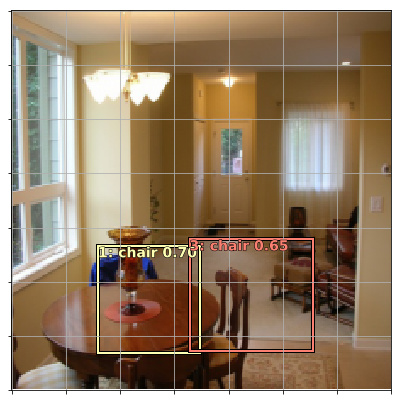
Thresholding seems important.
Am I on the right path? I’m still not sure if I’ve made all the changes to arrive at the right result.
The notebook is here (fastai_notes/experiments/notebooks/pascal-multi-without-background-in-conv-exercise.ipynb at master · binga/fastai_notes · GitHub). See In [103]: & In [104]: code blocks.
2 Likes
I don’t have time to look at the notebook now, but it looks on the right track. Try running it with focal loss and nms and see how it goes.
For bonus points, try to implement mAP metric and compare.
When I set bias value to 0, I needed to train longer with bit higher LR to get similar val_loss.
When I checked the bias values(just print head_reg4.out.oconv1.bias ) after training, they are between -3.9 and -3.4. Bias values were moved from 0 to around -3.x by training, so I guess they need more training or higher LR (than when moving from -3 to -3.x)
Interestingly, when I put bias value of -3.5, final bias values were more tight - between -3.510 and -.3552
I thought any reasonable bias should be okay since NN will figure out, but it looks like it’s good to have good starting value (at least if I want quick convergence)
BTW, these experiment is from a case that k=1. I had a same question and did this experiment.
3 Likes
OK now can you figure out why something around -4 might be a good starting point? Happy to give hints as needed.
Hey Jeremy…
In the OutConv class, the output conv layers are defined like this.
            self.oconv1 = nn.Conv2d(nin, (n_class)*k, 3, padding=1)
            self.oconv2 = nn.Conv2d(nin, 4*k, 3, padding=1)
So I figured that it is equal to the following line of the paper with k=4
![]()
Then I used following Conv layer calculations to find output detections.
-
38x38x512 ---------> 3x3x512, 4 filters, P=1, S=1 --------------> 38x38x4 = 5776
-
19x19x1024 ---------> 3x3x1024, 6 filters, P=1, S=1 -------------> 19x19x6 = 2166
-
10x10x512 -----------> 3x3x512 , 6 filters, P=1, S=1 -------------> 10x10x6 = 600
-
5x5x256 ------------> 3x3x256, 6 filters, P=1, S=1 -------------> 5x5x6 = 150
-
3x3x256 ------------> 3x3x256, 4 filters, P=1, S=1 -------------> 3x3x4 = 36
-
1x1x256 ------------> 3x3x256, 4 filters, P=1, S=1 -------------> 1x1x4 = 4
Total = 8732
What I did was alright ?
Somehow I couldn’t repro bias converging around -3.5 again with starting bias 0.
While debugging this, I noticed that class loss is x72 higher than BB loss (when bias is 0 and k=1).
I guess this makes lr_finder suggest high LR, but this high LR causes BB prediction branch to jump around.
When I set bias to -4(-5 seems to bit better), class loss becomes only x4 of BB loss and two prediction branches are reasonable to have same LR.
Another way seems to be putting extra weight to one of the loss as done in pascal.ipynb’s detn_loss().
I checked SSD paper about this, and they mentions weight term α to balance to two losses (though they just set it to 1)
Is it this correct direction?
1 Like
Oh, it was my bad. In the previous cell I typed x, y = next(iter(md.val_dl)) instead of x, _ = next(iter(md.val_dl)) and therefore overwritten defined above y = learn.predict()
Thanks for the reply!
As we say in Russia “To solve the problem heroically, we must first create this problem heroically” =)
2 Likes
Yes that will help - although with focal loss I found a multiplier isn’t necessary.
My question really was: why is around -4 the right number? It may be obvious to you already, but just to explain this: the reason is that on average the random weights are zero, so the average activation before any training equals the bias. Most output activations will represent background in the final solution, which means they’ll have an output probability pretty low (around 0.02 or less). The final activation goes through a sigmoid, so we undo that using its inverse, the logit:
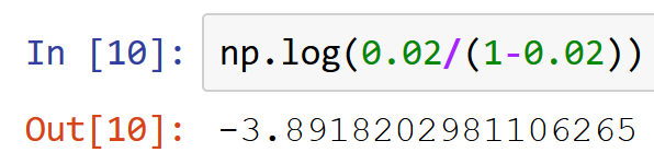
7 Likes
So that’s why! I have been wondering all week long where you pulled the -4 from.
I’ve been trying to implement the mAP loss Jeremy talked about and was wondering if I was doing it right. It begins the same way as the ssd loss, then I loop through all the ground truth objects to see how many times they have been detected with the right class.
def mAP_1sample(b_c,b_bb,bbox,clas):
    bbox,clas = get_y(bbox,clas)
    a_ic = actn_to_bb(b_bb, anchors)
    overlaps = jaccard(bbox.data, anchor_cnr.data)
    gt_overlap,gt_idx = map_to_ground_truth(overlaps)
    pos = gt_overlap > 0.4
    pr_act, pr_clas = torch.max(b_c,dim=1)#Convert our predictions into labels.
    tp = np.zeros(n_clas)
    fp = np.zeros(n_clas)
    fn = np.zeros(n_clas)
    for i in range(clas.size(0)):
        #Ground truth object i is detected if it's in gt_idx (it can be detected multiple times).
        #We check if those detections go with the right class prediction
        cl = clas[i].data #the class we are trying to detect.
        detect = ((gt_idx[pos]==i) * (pr_clas[pos].data==cl)).sum()
        if detect == 0:
            fn[cl] += 1
        else:
            tp[cl] += 1
            fp[cl] += detect - 1
    ap = tp/np.where((tp+fp) > 0, tp+fp,1) #To avoid a division by zero
    recall = tp/np.where((tp+fn) > 0, tp+fn,1) #Just if we want this one as well.
    return ap.mean()
If I understood correctly:
- false negatives: number of ground truth object not detected at all
- true positives: number of ground truth object rightly detected
- false positives: number of predictions of a given ground truth object minus one.
Does that sound right?
1 Like
To clarify - I meant to suggest you use it as a metric, not as a loss. You would use the metric after the nms step to test the end-to-end effectiveness of your trained model.
I believe that this is how most model results are presented in papers and evaluated in competitions.
Looks like you got it! ![]()
1 Like
Sorry, I meant metric, not loss. Also I hadn’t understood that we have to sum all true positives/false positives other all the pictures of the validation set before applying the formula for AP/mAP so the code above won’t work.
I’m not quite sure I understand the definition of false positives though, and searching on the net has made me even more confused. When we have five predictions with the right class for ground object number one, I gather it’s one TP and four FP, but how do we count a prediction for a ground truth object that doesn’t give the right class?
For instance, let’s say I have a ground truth object of class one for which I have 5 predictions, 3 of class one, 2 of class two. How many false positives does that give? 4?
I’m unable to prevent overfitting. The train_loss is much lower in comparison to what it was without making the background removal change for an almost the same validation_loss.
Is anyone else able to bring the validation_loss below 10?
I am having trouble understanding how the “find bounding boxes AND labels” section works. In particular,
tfms = tfms_from_model(f_model, sz, crop_type=CropType.NO, tfm_y=TfmType.COORD, aug_tfms=aug_tfms)
md = ImageClassifierData.from_csv(PATH, JPEGS, MBB_CSV, tfms=tfms, continuous=True, num_workers=4)
we set things up to find bounding boxes – with tfm_y=TfmType.COORD and continuous=True, but then we shove the category ID into the dataset as well. How does the model know that it should not treat categories as continuous, or do COORD style transforms on the categories?
The bounding box dataset doesn’t get modified, only added to.
That answer didn’t make sense to me until I realized that it did IFF the effects of tfm_y and continuous have no effect after the from_csv() call happens, and then it makes perfect sense.
I don’t fully understand what tfm_y and continuous do, which is I think at the root of my problem. (That’s probably from working on refugees instead of part1v2 homework, sorry.)
1 Like