Part 2 Lesson 9 wiki

This is really cool. And I really like how this seems to be an evolution of the idea in the multibox paper where I think they clustered all bounding boxes coordinates and instead of having the network predict those just had the NN predict the residuals (I think that’s what they did but might be wrong).

This whole idea with clustering and residuals is really neat and it seems to me a NN might be better suited to refine something vs outputting it from scratch (unsubstantiated claim warning). I am not sure we will get around to looking into this this time around but from watching part 2 v1 I saw Jeremy cover mean shift clustering and approximate versions of algorithms. Hoping to go study that at some point should I ever get a chance :slight_smile:

1 Like

Take a look at this @alessa :wink: I think I’ll link to it from the wiki of the lesson - was also looking for this piece of information quite extensively :slight_smile:

1 Like

Thanks Radek. It makes more sense.
Also it is the easiest way to add a vector full of zeros - because you want to minimize the loss - make the values as closest to zero. But if there is also a 1 representing the background - you want to minimize that as well. So I think it is the easiest way to add a new class, and still not using it in the end when you want to minimize the loss.

This is the hardest fastai lecture I have ever encountered, but I must say the supplementary materials people shared and the discussion in this thread have been amazing and of immense help.

Thx to all that participated!

Looking forward to getting to the bottom of what is happening in the notebook over coming days :slight_smile:

4 Likes

It’s a lot of material. I’m about 1/3 through the notebook and have been trying to work through it. My goal is that by the time we get to lesson 14 I am at a point where I am fully comfortable with the current ideas and ready to enhance things.

2 Likes

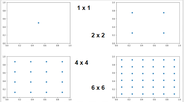
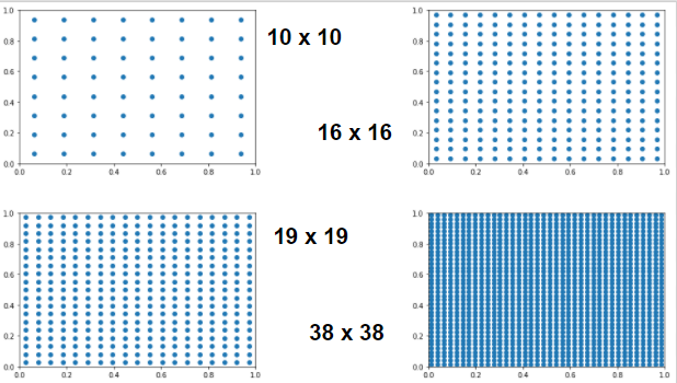
Visual Intuition - Understanding the impact of anchor grid size change - 1x1, 2x2, 4x4, 6x6, 10x10, 16x16, 19x19, 38x38

Question - When grid size is 38x38 (contains few pixels) or grid size contains just 1 pixel does it has the intuition of object segmentation where the prediction is at the pixel (few pixels) level? Is this understanding correct?

image

image

2 Likes

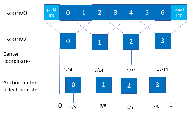
In lecture notes, the anchor box’s center cooridnates for 4x4 cells are (1/8, 3/8, 5/8, 7/8).
(For simplicity, only X coordinates are listed in [0,1) coordinate)
But I think the actual center is more like (1/14, 5/14, 9/14, 13/14)

Backbone model’s output is 512x7x7 and sconv2 is Conv2D with stride 2, padding 1.
So sconv2’s output will be alinged like below diagram, and the center of each cell is slightly different from one from lecture note.
ssd_anchor

The difference is .054(12 pixels) in the edge area, and .018(4 pixels) in center area.
It may be not much error and but I guess it can still impact the performance especially object in edge area.

And if we consider imbalanced padding/pooling in backbone model(last column/row are dropped during 2x2 pooling when # of column/row is odd), the center coordinate can be skewed bit more.

Let me me know if I misunderstood something. I’ll experiment with new center coordinates later.

1 Like

That’s how I understand segmentation. I’d be interested to hear from somebody that knows more about it.

In the papers they don’t seem to have their anchor boxes exactly match the conv grid. I think there are benefits to having the anchors be evenly spaced the way we’re doing it, but I haven’t tested. Will be interested to hear what you find if you experiment.

More time I spend understanding it, more confuse I get. Is the minute 01:08 where Jeremy is saying that:

a lot of papers talk about it (...) trying to predict a background category using a softmax is really hard to do, what if we use binary cross-entropy instead?

Isn’t the softmax output (probabilities) - the input for the cross-entropy?
How can we use binary-cross-entropy instead of softmax? And then what will be the input for the cross-entropy? Will we use sigmoid-output instead?

Thanks for the patience :slight_smile:

I think you are on the right track.

Softmax output with cross entropy cost => one question, which out of the n classes does this object belong to? probabilities sum to 1

n sigmoid outputs with binary cross entropy cost => n questions, is this object of class 0? is this object of class 1? etc Can be used with multiple labels and also we no longer have to ask our NN to identify background, which the idea is that it might be easier to do for the NN then learning a whole new class for ‘there is nothing here’

  • Logistic function (sigmoid function is a special case of logistic function) and softmax function can be defined as “score functions”. They output real value(s) in the range (0, 1).
  • Logistic function assumed that the labels were binary. Softmax function is the generalization of the logistic function that allows us to handle K classes instead.
  • Logistic loss (a.k.a. binary cross-entropy loss) and (categorical) cross-entropy loss are loss functions. It uses to find the difference between the prediction versus the ground-truth label.

For example, for binary logistic regression with ground truth label \mathbf{y} \in \mathbb{R}^2, we use logistic function + binary cross-entropy (BCE) loss:

\mathbf{z} = \mathbf{Wx + b} \\ \hat{\mathbf{y}} = \text{logistic}(\mathbf{z}) \in \mathbb{R}^2 \\ \mathcal{L}_{\text{BCE}}(\mathbf{y}, \mathbf{\hat{y}}) = - \sum_{k=1}^2 y_k \log \hat{y}_k \in \mathbb{R}

For multinomial logistic regression (a.k.a. softmax regression) with ground truth label \mathbf{y} \in \mathbb{R}^K, we use softmax function + (categorical) cross-entropy (CE) loss:

\mathbf{z} = \mathbf{Wx + b} \\ \hat{\mathbf{y}} = \text{softmax}(\mathbf{z}) \in \mathbb{R}^K \\ \mathcal{L}_{\text{CE}}(\mathbf{y}, \mathbf{\hat{y}}) = -\sum_{k=1}^{K} y_k \log \hat{y}_k = - \mathbf{y}^T \log \hat{\mathbf{y}} \in \mathbb{R}

Note that \mathbf{y} is an one-hot encoded ground-truth vector.

2 Likes

hi @radek my understanding is that, in an image, we have multiple objects to be detected.

Each object in the image is a multi-class classification problem, so the obvious choice should be to use softmax for each object and then use cross-entropy to calculate the loss.

“n sigmoid outputs with binary cross entropy cost =>”, so why do u make this statement. Is there a role for sigmoid function and binary cross entropy in this multi-object multi-class detection?

There must be something obvious here but i am not getting the intuition behind using n sigmoids.

I am trying to clarify my fundamental discomfort with loss calculation.

It is all about how you frame the question. Lets consider a single anchor box where we want to classify if it belongs to one of the categories (person, bottle, etc). If we have 20 classes, we can ask our NN 20 questions - is this a person? is this a bottle? is this a table? etc. If the network answers no to all these questions (probability of class below certain threshold value), then this implies that we are looking at an anchor box of class bg. But we never asked our NN to learn to predict the background class!

Alternatively, we could have 21 outputs (20 classes + 1 extra class for bg) and ask a question using softmax - which is the class associated with this anchor box? Asking this question would require our NN to learn to predict the bg class! This, as far as I understand, is considered a harder question to ask. I have not gotten to the point where I have played with this (I will!) but I would guess that people ran experiments and using sigmoid activations with binary cross entropy loss turned out to work better.

3 Likes

download

Why do we divide by 2 here? If I understand correctly, we are doing this to limit the offsets to max 0.5 the width / height of the grid cell?

1 Like

davidluo has written down a step-by-step guide of SSD loss that you may be interested of it.

According to his note:

# activation bb's center (x,y) can be up to 1/2*grid_sizes offset from original anchor box center
actn_centers = (actn_bbs[:,:2]/2 * grid_sizes) + anchors[:,:2] 

# activation bb's height and width can be between 0.5-1.5x the original anchor box h&w
actn_hw = (actn_bbs[:,2:]/2+1) * anchors[:,2:] 
2 Likes

Each predicted BoundedBox can be moved by 50% of a grid size from where its default position is, and the size can be up to twice as big If it makes sense

1 Like

Confused about my results, and looking for guidance.

My big difference is that I am forced to use a batch size of 32 because of my old GPU.

My results are all over the place when compared with Jeremy’s.

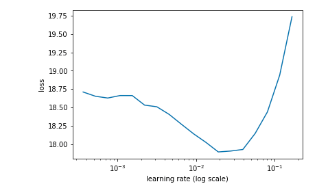
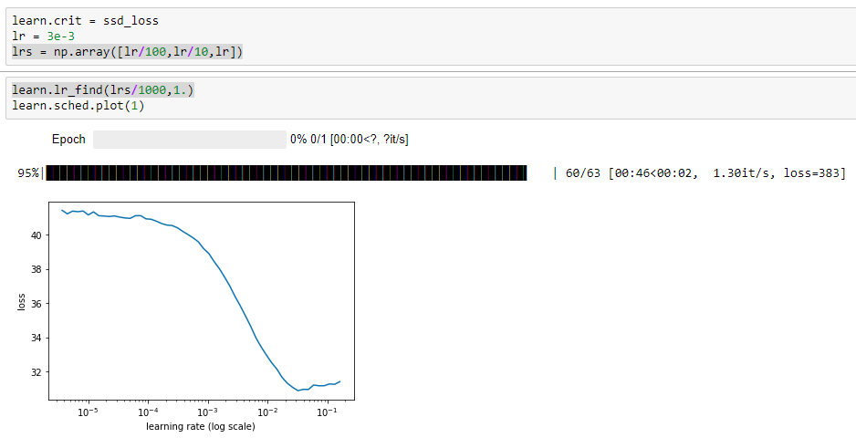
For instance after the initial learn.model() and the application of lr = 3e-3, lrs = np.array([lr/100,lr/10,lr]), learn.lr_find(lrs/1000,1.)

My plot:

Jeremy’s plot:

Then after learn.fit(lr, 1, cycle_len=5, use_clr=(20,10))

My results:

epoch      trn_loss   val_loss                                                                                         
    0      19.368023  15.716943 
    1      15.620254  14.04254                                                                                         
    2      13.78509   13.574283                                                                                        
    3      12.395073  13.149381                                                                                        
    4      11.260969  12.904029                                                                                        

[12.904029130935669]

Jeremy’s:

epoch      trn_loss   val_loss                            
    0      43.166077  32.56049  
    1      33.731625  28.329123                           
    2      29.498006  27.387726                           
    3      26.590789  26.043869                           
    4      24.470896  25.746592                           

[25.746592]

Well, this looks good at this stage, but why is everything roughly half / twice?

But after all of the next process of testing, creating more anchors, then the Model section we come to:

learn.crit = ssd_loss
lr = 1e-2
lrs = np.array([lr/100,lr/10,lr])
x,y = next(iter(md.val_dl))
x,y = V(x),V(y)
batch = learn.model(V(x))
batch[0].size(),batch[1].size()
(torch.Size([32, 189, 21]), torch.Size([32, 189, 4]))
ssd_loss(batch, y, True)

I end up with this:

Variable containing:
 164.1034
[torch.cuda.FloatTensor of size 1 (GPU 0)]

Jeremy has:

Variable containing:
 4.5301
[torch.cuda.FloatTensor of size 1 (GPU 0)]
 Variable containing:
 61.3364
[torch.cuda.FloatTensor of size 1 (GPU 0)]

Variable containing:
 65.8664
[torch.cuda.FloatTensor of size 1 (GPU 0)]

Only one Variable in my notebook?

After learn.lr_find(lrs/1000,1.), learn.sched.plot(n_skip_end=2), and plot I have:
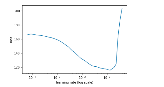
image

Jeremy has:
image

With learn.fit(lrs, 1, cycle_len=4, use_clr=(20,8)) I have:

epoch      trn_loss   val_loss                                                                                         
    0      72.285796  57.328072 
    1      57.207861  48.549717                                                                                        
    2      48.630814  44.12774                                                                                         
    3      43.100264  41.231654  

Jeremy has:

epoch      trn_loss   val_loss                            
    0      23.020269  22.007149 
    1      19.23732   15.323267                           
    2      16.612079  13.967303                           
    3      14.706582  12.920008                           

[12.920008]

After that I do my best at adjusting the lr (and subsequent lrs) and use_clr
e.g. tried lr = 1e-3, tried use_clr=(60,10) and got this upon retesting lr:
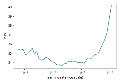
image

But the best I’ve achieved is this and I’m just spinning my wheels:

epoch      trn_loss   val_loss                                                                                         
    0      33.419068  39.042112 
    1      32.294365  38.817078                                                                                        
    2      31.792605  38.655365                                                                                        
    3      31.260753  38.581855 

ANY ADVICE ANYONE?

That all looks fine. I don’t run my notebook in order so you shouldn’t expect the same results. Losses depend on # anchors so you and I likely used different numbers.

Focus on the pictures! See if your bounding boxes and classifications look reasonable.

OK, thanks Jeremy. I will carry on - I used these combinations for anchors:

anc_grids = [4,2,1]
anc_zooms = [0.7, 1., 1.3]
anc_ratios = [(1.,1.), (1.,0.5), (0.5,1.)]

Can you please explain the difference in Variable count at the end of running ssd_loss?

It seemed amazing to me that I could start and finish at such a high error rate compared with you, and I experimented with increasing the first parameter of use_clr as there was so much more difference between the points on my learning rate graph - not sure if I have understood that properly…

UPDATE:
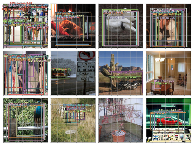
I carried on, and got as far as displaying bounding boxes in the code section just after learn.save('prefocal') - the result below. Unfortunately the next time I ran the learning rate finder my GPU crashed. I know it’s way past time I upgraded from a 2GB GPU - its not worth the time and effort to juggle with these tiny resources :frowning: