Meet BatchLossFilter: a new technique to speed up training

[oguiza (Ignacio Oguiza)]

I’d like to share with you a new callback I’ve created that has worked very well on my datasets.

Last week @Redknight wrote a post about this paper: Accelerating Deep Learning by Focusing on the Biggest Losers.

The paper describes Selective-Backprop, a technique that accelerates the training of deep neural networks (DNNs) by prioritizing examples with high loss at each iteration.

In parallel I also read a tweet by David Page:

Those idea really resonated with me. I’ve always thought that it’d be good to spend most of the time learning about the most difficult examples. This seemed like a good way to do it, so I decided to try it.

The paper’s code base in Pytorch is publically available here.

However, I thought I’d rather implement the idea with a different approach. The idea is very simple: identify those items within each batch that are responsible for a given % (I chose 90%) of the total batch loss, and remove the rest. In this way you force the model to dynamically focus on the high loss samples. The percentage of samples remaining will vary per batch and along training as you’ll see.

So I’ve created a new callback (BatchLossFilterCallback).
It’s very easy to use this technique. The only think you need to do is to build your DataBunch, model and learner and usual, and then:

learn.batch_loss_filter()

That’s it!

I’ve run the callback in CIFAR10, and have shared a notebook within the fastai_extensions repo.

Here these are the test results:

1. Time to train (100 epochs): 15.2% less time to train (in spite of the additional overhead)

2. Accuracy: same as the baseline model (at least in 100 epochs)

However, training is smoother, and there’s a significant different in terms of validation loss. I believe that with a longer training there could be a difference in accuracy. But I have not confirmed this yet.

3. Validation loss: lower and smoother.

4. Selected samples per batch: This is very interesting in my opinion, as it shows the % of samples that make up 90% of the total batch loss. As you can see, 90% of the total loss is initially made by a large % of batch samples, but as training progresses, it dynamically focuses on the most difficult samples. This samples are not necessarily the same all the time, as they are chosen for each batch. In the end, the model will be focused on 12% of the most difficult samples. This is why training takes less time.

Note:
There are actually 2 hyperparameters: min_loss_perc: select samples that make a at least that %, and min_samples_perc: select at least a given % of highest losses. Both can be used at the same time. In my case I just used min_loss_perc.

If you decide to try it, just let me know what you think!

EDIT:
I’ve run the same tests with 200 epochs and the results are pretty similar.

• Training time: 15% reduction (using min_loss_sample=.9)
• Accuracy: same (95.03% for baseline and 95.15% for BatchLossFilter)
• Lower validation loss: BL .281042 vs .182068 for BatchLossFilter
• Selected batch sample percent at the end of training: 13%

So it seems this approach makes the model more certain when it’s right, achieving the same accuracy.

[muellerzr (Zachary Mueller)]

AWESOME! I’ve been pondering trying to do this since I first heard about it! I’m excited to try it out Thanks @oguiza Well done!

[oguiza (Ignacio Oguiza)]

Excellent!
Please, let me know how it works! In principle, the callback should work on any type of datasets.

[bwarner (Benjamin Warner)]

I immediately tried to use the callback with to_fp16() and it broke, so I created a pull request to add support for mixed precision training.

I also added an option mixed_precision_batch:bool=False which rounds up each batch to the nearest multiple of eight for optimal tensor size for mixed precision.

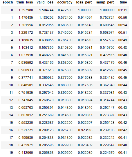
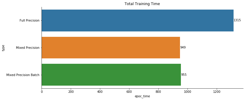
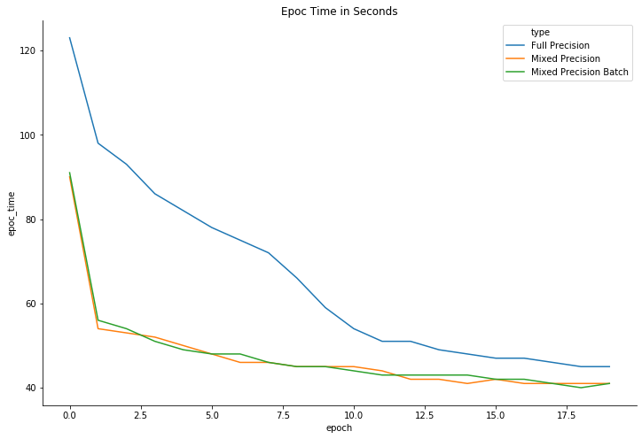
I ran a similar cifar test on a Tesla T4 for 20 epocs in full and mixed precision. Despite using 24 cpu cores, the mixed training was cpu limited. Further testing is needed to see if the mixed_precision_batch option is worth using.

model = models.WideResNet(num_groups=3, N=4, num_classes=10, k=2, start_nf=32)

learn = Learner(data, model, metrics=accuracy).batch_loss_filter(min_loss_perc=.9)

learn = Learner(data, model, metrics=accuracy).to_fp16().batch_loss_filter(min_loss_perc=.9)

learn = Learner(data, model, metrics=accuracy).to_fp16().batch_loss_filter(min_loss_perc=.9, mixed_precision_batch=True)

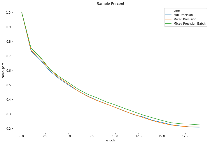
As you’d expect, mixed_precision_batch training has a higher loss percent than normal training.

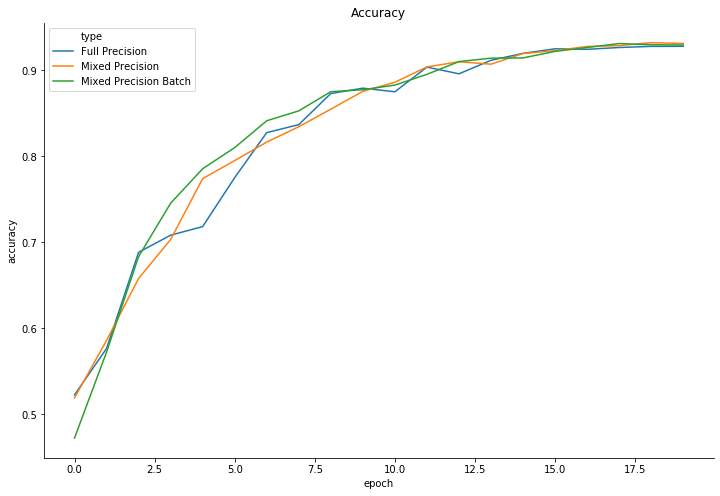
The three modes of training all look very similar otherwise (outside of time).

Currently the callback doesn’t work when predicting n>1 classes, either with flattened loss or non-flattened loss. I plan on taking a look into that in the near future.

[TomB]

Nice work Ignacio, was looking at implementing something along the lines of this paper after seeing it.

Despite using 24 cpu cores, the mixed training was cpu limited.

What makes you think it was CPU limited? Was it maxing CPUs or not fully utilising GPU?

From looking at the code it may be that the implementation is non-optimal in terms of CPU<->GPU transfers. It looks like at the start of each batch it’s running a forward pass on the data to get losses and moving the loss back to the CPU (this is hidden in the np.array(self.crit(self.model(last_input), last_target)) which will call fastai’s monkey=patched Tensor.__array__ which moves GPU tensors to CPU). So on top of the overhead of two forward passes on every batch there’s the latency of moving a batch back from the GPU to the CPU.
In fact looking at the CPU usage may not give an accurate picture here as it may consider the waiting that has to be done in .cpu() as CPU usage when it’s not really limited by CPU power it’s got to wait around a lot in CPU code. The torch.autograd.profiler may give a slightly better picture here (think it still counts as CPU time but show it’s in .to() (or similar)).

Not to attack Ignacio here. It’s not obvious to me how best to implement this idea in the paper, with performance issues in most approaches. Double forward and early access of GPU results in the implementation here. Wasted forward in the straightforward implementation of the paper where you forward everything then drop items for the backward, and possibly early access of forward loss to decide to drop batches. Or, in the implementation suggested in the paper where losses are cached you have extra memory overhead on the GPU if you try the more efficient route of doing it all on GPU (which may be tricky with more limited GPU operations compared to numpy). Or if you try to move to CPU to avoid extra GPU memory usage then you have possible issues with waiting for transfers there.
This is also complicated by the fact that it depends on what other things are doing. There’s various places where fastai accesses GPU data right after creation so those are already slow points and the more important thing may be reusing those not adding more (this also potentially depends on what callbacks ar used if they access stuff).
It may actually be that in the context of fastai the original implementation of doing a forward on everything before then dropping stuff for backwards is better. For smoothing and recording losses fastai already moves losses back to CPU so there’s a pause there. If you can implement it within this pause (while avoiding extra pauses) then there may not be any extra overhead on top of fastai’s.

[oguiza (Ignacio Oguiza)]

Hi @bwarner, thanks for using the callback and providing feedback!
I had not tested mixed precision, and I happy to add support once you clarify what’s the best way to do it.

Currently the callback doesn’t work when predicting n>1 classes, either with flattened loss or non-flattened loss.

I guess you mean that your modified callback doesn’t work yet, since the original one does support multiclass (CIFAR10).

Please, let me know if you clarify how it should be modified to support mixed precision.

[oguiza (Ignacio Oguiza)]

I’ve run one more test using BatchLossFilter (BLF) in combination with Mixup.
The results were a bit surprising to me.
In summary BatchLossFilter doesn’t help in combination with Mixup. Time to train, accuracy and validation loss were worse when used in combination with BLF.
I think the key lies in how does a model using Mixup learns.
Let’s take a look at the chart that represent the % samples that make up 90% of the total batch loss:

During training BLF started to behave as expected, reducing the % of samples passed. But a bit later, the opposite started to occur. There were more samples in that 90%.
The way I interpret this is that when training with mixup the model learns from average (mixed, noisier) samples with lower confidence.
Since samples may be mixed with any other sample, there are not easy or difficult ones, and thus all are equally easy/difficult, resulting in a similar loss for all of them.
Without mixup at the end of training, 90% of the loss came from 13% of the samples, while with mixup 90% of the loss comes from 86% of the samples. I think this is what helps generalize better.

Based on this, I think BLF may be useful to speed up training (as long as single samples are used, and not combinations of samples like in mixup) or if you need a higher level of confidence in the correct samples. But if you want to achieve a higher generalization and better accuracy, mixup, cutmix, etc seem to be a much better approach.

[TomB]

Or presumably for cases where mixup can’t be applied (or at least not the fastai implementation). Haven’t investigated deeply but don’t think you can use mixup for segmentation but BLF should work fine.

[maral]

It would be interesting to try a slight permutation. Given the distribution of errors take the top-N and bottom-N samples in the distribution for each batch. I have a hunch this will help the learner discriminate faster.

[TomB]

Interesting idea to try.
Another thing, which kinda of generalises that idea a little, might be to introduce some curriculum learning based ideas. This could be as basic as scheduling the min_loss_perc/min_sample_perc across training. So initially more easy samples gradually favouring harder as training progresses.
Think that sort of scheduling of arbitrary hyper-parameters is something that’ll be a lot easier in fastai v2, but there is some generic scheduling stuff in v1.

There seems to be some slight evidence of an initially lower performance of BLF after which it catches up in the results shown. And this very intiial stuff can sometimes be hard to pick up in fastai given the tendency to pretty high learning rates compared to other libraries, offset by various little optimisations and controls (especially heavy regularization).

[davidpfahler]

I don’t know if this has been proposed before, but as far as I can see it’s not what this paper does: Wouldn’t it make sense to also alter the learning rate schedule depending on whether we are looking at top losses or bottom losses? Or am I off base here?

E.g. if we start with easy examples like @TomB suggested and gradually introduce harder ones, shouldn’t we also reflect that in the learning rate schedule?

[TomB]

Yeah, that sounds like another good idea.
Also probably the sort of thing that would be hard for the paper to really address. Given the focus on presenting one core novelty and the difficulty of fully validating in even just one base case.

[TomB]

Also, anyone tried it on the imagenette/imagewoof datasets? Part of Jeremy’s reasoning for these was that cifar isn’t always a great indication of success on more standard data (the tiny images representing a rather unique challenge). Not sure I’ll have anything else ready to occupy my GPU tonight so can try it out if it hasn’t been done.

[oguiza (Ignacio Oguiza)]

anyone tried it on the imagenette/imagewoof datasets?

No, I haven’t run any other tests outside CIFAR.
It’d be great if you run any test on other datasets

[TomB]

OK, I’ll look to try that then.
Thinking about it a bit more, imagenette/imagewoof might not really be the best here. Given they both aim to create subsets of a given difficulty they’re not necessarily the best thing for testing a difficulty based approach like BLF. But we’ll see. There should still be a difficulty distributions in them for BLF to exploit.

[bwarner (Benjamin Warner)]

I guess you mean that your modified callback doesn’t work yet, since the original one does support multiclass (CIFAR10).

Sorry, I didn’t state that clearly. The callback doesn’t work when predicting multi-label images, when fastai creates a MultiCategoryList. If there’s six labels per image, then flattened loss returns an array of length batch size * 6 with losses per label. Would need to reshape the output to [bs,6], which is the same output from non-flattened loss, and then sum the per-label loss before picking the top n percent loss images as the callback currently does. The dataset I am currently working on is multi-label, so I plan on looking into this soon, as I think BatchLossFilter could work well with it.

The changes I made to support mixed precision implementation works with multiclass datasets such as CIFAR10. It’s the dataset I ran my tests on. I added another commit to my Pull Request which exports the callback to the nb_BatchLossFilter.py.

What makes you think it was CPU limited? Was it maxing CPUs or not fully utilising GPU?

During the mixed precision training the GPU usage decreased from in the mid-to-low 90 percent to upper 50 percent while CPU usage stayed the same at mid-to-upper 80 percent the entire run. If I thought to query nvidia-smi during training that would have made an interesting chart.

[JoshVarty]

Thanks for your implementation! I’ve been playing around with it but I’m missing drop_cb_fn(). Where is this imported from? I can’t seem to find a definition in your extensions repository or in the fastai repository.

[muellerzr (Zachary Mueller)]

On ImageWoof, I tested briefly on a 5 epoch and I didn’t see any change. I imagine perhaps we need more 10-50 (large range I know) to see the results?

[oguiza (Ignacio Oguiza)]

Hi @JoshVarty,
Sorry about that! It should be fixed now. Please, try it and let mw know if it works.

[oguiza (Ignacio Oguiza)]

I would think you would start to see a performance (speed) improvement after more epochs. Same_perc selected (shown in metrics) needs to be below .5 more or less to start to see an improvement, and that takes more epochs.
It’d be good to confirm if you get the same type of results I get: lower validation loss that doesn’t translate into higher accuracy.