What a simple, elegant idea!
Q: If you allow BatchLossFilter to train for the same amount of time as the plain model, does BatchLossFilter get better accuracy than the plain model?
What a simple, elegant idea!
Q: If you allow BatchLossFilter to train for the same amount of time as the plain model, does BatchLossFilter get better accuracy than the plain model?
Yes, if the model was not fully trained. Essentially what we have here is a way for us to speed up how to achieve a maximum accuracy from the same model/technique. So for instance one experiment with the ImageWoof as stated above is I’ll be looking more towards can we achieve the maximum in 80 epochs faster (even though at 80 epochs should be roughly the same as that cut off).
This sounds pretty much identical to hard negative mining where you backpropagate only highest loss items from the batch.
Yeah, you are probably right. However, there are some differences discussed in this twitter thread.
What exactly do you mean by no change? Presumably if you saw the same accuracy after five epochs that would be a win for BLF as that would mean it achieved the same results with fewer items and less wall time.
I haven’t seen the results, but I’m not sure there will be any gain in terms of time with so few epochs. It may even be the opposite, you might see a time increase.
The reason for that is the additional overhead. BLF saves time if the % of batch samples passed is significantly reduced (50% or less). That’s why when you run it for some few epochs, or the loss is almost the same across all samples (like in the case of mixup) you may not see any benefit. I think this is clearer in this chart:
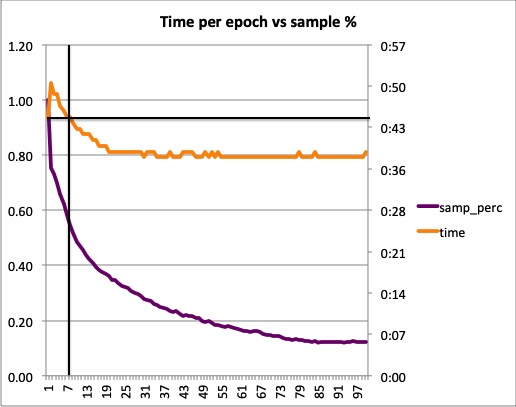
In this case, there is a benefit after 7 epochs or so.
Ah yes, I was missing the fact that it only really starts doing less per epoch as training goes on. Nice chart, thanks.
The other interesting chart for evaluation might be accuracy vs. wall-time. Or, as is often used in performance optimisation, time to a certain accuracy.
When looking at some ideas this work prompted I came across Not All Samples Are Created Equal: Deep Learning with Importance Sampling. Might be interesting, and links into the importance sampling literature which looks like another approach to this problem. Coming from a more maths heavy approach to DL (talk of convex optimisation is a good sign I’ll struggle). But there’s code for it at https://github.com/idiap/importance-sampling, for keras though. With the technique they train vgg19/mnist/CPU to ~0.65% error in 1m41s versus 9m23s with standard uniform sampling (there’s comparisons with resnets on cifar10/100 and on fine-tuning an imagenet pre-trained resnet on cifar too, that one was just easy to state).
Of note here, they claim using “the loss to compute each sample’s importance … is not a particularly good approximation of the gradient norm” (p.1). The upshot I gather being that loss is not a very good predictor of how much a network will learn from a particular sample which is what you really want to maximise (but computing the gradient norm is intractable, the contribution here is to efficiently compute a bound on it to use instead).
EDIT: Just noticed this paper is what the SelectiveBackprop compares to, claiming higher performance. However, if you look they actually say they compared to “our implementation of Kath18 (Katharopoulos & Fleuret, 2018) with variable starting, no bias reweighting, and using loss as the importance score criteria” (p.6, emphasis mine). But I think the primary contribution of Kath18 is their gradient-norm bounding as a superior alternative to loss. So this seems an odd comparison to make (to say the least).
No worries, I’ll give it a shot this afternoon.
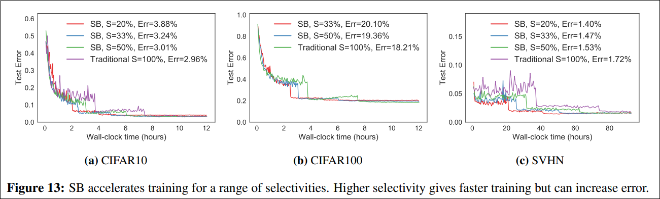
One interesting thought I had related to Figure 13 which shows the effect of using different selectivities (β) when choosing examples:
Higher selectivities give faster training but increase error. Perhaps it would be possible to anneal the sensitivity to try to get the best of both worlds. We could start with a high selectivity and decrease it as training progresses?
This would probably only work if the early training runs don’t put the network in a bad state from which is cannot recover.
Of note here, they claim using “the loss to compute each sample’s importance … is not a particularly good approximation of the gradient norm” (p.1).
Interestingly, the linked paper Accelerating deep learning by focusing on the biggest losers paper makes the opposite claim:
We suspect, and confirm experimentally, that examples with low loss correspond to gradients with small norm and thus contribute little to the gradient update.
Their justification seems to be:
Our experiments show that suppressing gradient updates for low-loss examples has surprisingly little impact on the updates. For example, we empirically find that the sign of over 80% of gradient weights is maintained, even when subsampling only 10% of the data with the highest losses (Fig. 5b). Since recent research has demonstrated that the sign of the gradient alone is sufficient for efficient learning (Bernstein et al., 2018), this bodes well for our method.
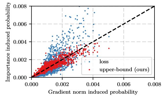
Interesting indeed. In Kath18 (p. 5):
We observe that our upper bound is almost perfectly correlated with the gradient norm, in stark contrast to the loss which is only correlated at the regime of very small gradients. Quantitatively the sum of squared error of 16,384 points in figure 2 is 0.017 for the loss and 0.002 for our proposed upper bound
(Not to argue either way, I certainly don’t understand the details enough to come down on either side)
If it is the case, as their paper suggests, that Jiang et al. (Accelerating Deep Learning) only tested the Kath18 approach with a loss measure implementation then comparison with the upper bound measure might be interesting.
Also, if the Jiang et al. comparison with Kath18 uses loss as the importance measure for both, then presumably the reported improved performance is a result of a better method for selection based on this measure. So it might also be possible to apply these advances in selection with Kath18’s purportedly better measure and improve on the results there.
Kath18 also develop a “metric to decide if the variance reduction is significant enough to justify using importance sampling” (p.4) so they avoid the overhead at the beginning when they claim it won’t help, only kicks in after what looks like a fair bit of training. Calculated based on the losses from standard, fully-backpropped, batches at the beginning it looks. Might work in the context of Jiang et al. too, think it’s based on the extra forward passes needed in both methods not the exact overheads of the other calculations (derived from an approximation of forward vs. backward time I gather). I think they still see benefits before this threshold it’s just when the method is guaranteed to help. But maybe a more stringent threshold could be derived from it.
I’m not sure about this. If you take a look at the first post on this thread, the validation loss was never really higher for BLF, and it was lower towards the end when using loss_perc=.9.
But I agree it may be interesting though to to leave loss_perc=0, and anneal sample_perc (selectivity threshold). Is this what you have in mind?
I think those comparisons are pointing out differences in the final error(/accuracy) at convergence which aren’t always reflected in the initial losses. In some cases (mostly it seems with higher selection proportions) there seems to be a drop in final accuracy with SelectiveBackprop in spite of the expected initial advantages in both loss and error.
Analyzing the code of the original article is a bit over my head. Can’t we write a custom loss function which in turn calls a regular loss function (like BCEWithLogits) with reduction set to ‘none’ and picks say the highest 90% and returns an average of these 90%. I wrote a function like this but didn’t notice any meaningfull drop in training time. I would expect this to be more effective late in the training, when most samples are “easy” for the netowrk.
@oguiza Slightly related to this technique, this one could be a more accurate way to achieve the selection…
Consistency regularization for generative adversarial networks: https://arxiv.org/pdf/1910.13540.pdf
Edit: Wrong paper, this is the right one
SMALL-GAN: SPEEDING UP GAN TRAINING USING CORE-SETS: https://arxiv.org/pdf/1910.13540.pdf
Thanks a lot for sharing @Redknight! I’ll read it during my Xmas break