Lesson 9 official topic

[johnowhitaker (Jonathan Whitaker)]

Looking into this and still haven’t quite figured it out but I have found a ‘fix’ that might hint at the issue. Setting start_step=45 or 47 (out of 50) you get a pretty good-looking result. But 46 is a noisy mess (bottom image here). Why 46? Why 4 iterations left? The LMS sampler keeps order previous predictions and the default is order=4. Switching the code to latents = scheduler.step(noise_pred, t, latents, order = 2).prev_sample for order=2 or (3, also works) and suddenly the result is fine (top). We could try to dig in and see exactly what is up, or you could switch to order=3 or order=2 which seem to avoid the issue (and 47/48 look fine with those too, plus from higher noise levels (lower start_step) I prefer the outputs using a lower order too - bonus day!

[brismith (Brian Smith)]

Good find - I was struggling to see ‘why 46’.

[bencoman]

@johnowhitaker

The LMS sampler keeps order previous predictions and the default is order=4.

I can’t quite articulate the link between this and the following, but this evokes in my mind an image of resonant feedback observed while tuning a PID process control loop.

The aim of PID control is minimise the error between a process variable and its control setpoint. A real-world system has a resonant timestep (the “ultimate period”) such that control action can cause sustained oscillations of process variables. This has a practical use as a field technique for tuning PID loops (https://www.youtube.com/watch?v=dTZnZZ4ZT7I) where the gain “Kc” is raised until resonant oscillations are observed, and from which optimum control parameters can then be inferred.

The tentative concept is that the training steps end up storing graduated shells of noise around the ideal-bird (point of minima-noise) - so the decoder is bouncing back and forth in the noise valley around the ideal-bird, rather than settling down into it. I wonder also if such a noise-valley somehow relates to the guidance-decay discussion in Lesson 10, in the same way a high learning-rate was shown in Part 1 to bounce across the optimsation valley.

I can’t quite connect the dots to determine if there is anything really pertinant about this line of thought or my subconcious is misleading me, but maybe the following will usefully jiggle the neurons of others wiser:

• https://www.youtube.com/watch?v=6OH-wOsVVjg
• https://youtu.be/IB1Ir4oCP5k?t=124 - The “integral” component of seems similar to “keeping previous predictions”, although
• https://www.youtube.com/watch?v=fv6dLTEvl74
• https://youtu.be/uXnDwojRb1g?t=316
• https://www.youtube.com/watch?v=n829SwSUZ_c

[Edit:] Having mused over this a bit more, just thought I’d summarise that the key thing was that certain periods of historical sampling may be harmonic and lead to overshoot.

[johnowhitaker (Jonathan Whitaker)]

I’ve seen ‘PID samplers’ talked about (nothing published yet) - an interesting train of thought! Control theory in university traumatized me a little but I’ll definitely check out those links and see if they dredge up any PID-related insights. Thanks for sharing

[bencoman]

@johnowhitaker

Control theory in university traumatized me

Me too. Side-bar: The great thing about Ziegler-Nichols method is that in practice it completely bypasses all the math. Just turn knobs, observe, back off a bit - somewhat equivalent to fastai’s learning rate finder.

[sswam (Sam Watkins)]

I’m watching the lesson 9B math of diffusion video, and wanted to share a simpler formulation of the “add some noise” function as far as I understand it. I think we’ve covered this in Jeremy’s lectures too, but anyway maybe it’s useful. The notation used in the papers is pretty hard to understand.

let x be the current state (image),
x’ the next state (noisier image),
n a unit normal distribution (the noise) with mean 0 and sd 1,
β a blend factor in (0, 1), where 0 gives no change and 1 total change to noise,
α = 1 - β, the corresponding blend factor seen from the other side; 1 gives no change and 0 total change to noise,
b = √β the weight given to the noise,
a = √α the weight given to the current state,

Note that a² + b² = 1,
so (a,b) would be (1,0), ~(0.7,0.7), (0,1) for no change, halfway, and full noise.

Then:

x’ = ax + bn

I.e. The next state is a weighted average or blend between the previous state and unit noise, such that the sum of the squares of the weights equals 1.

This choice of blend function reminds us of Pythagores’ theorem, and is appropriate for blending perpendicular / orthogonal / uncorrelated values, like a clock hand turning from 12 o’clock to 3 o’clock, 0° to 90°, goes through a point sin(45°), cos(45°) = √0.5, √0.5 ≈ 0.7, 0.7, or blending red and green to make “rainbow yellow” (with 0.7 red and 0.7 green). I guess noise is uncorrelated with everything, so that makes sense.

[sswam (Sam Watkins)]

I made a slightly different “parrot diff”, with 50% grey indicating no change.

The notebook is here: https://sam.ucm.dev/ai/diffusion-nbs/Stable%20Diffusion%20Deep%20Dive.ipynb

Also I realised while watching lesson 9B closely that the vae decoder is not deterministic, it returns a “sample” where some pixels vary by up to 0.2% (in this case), i.e. 0.512 of a colour step with 8-bit color. This is an amplified difference between two samples (decoding the same macaw latent):

I checked and it seems that the vae encoder isn’t deteministic either, produces slightly different latents each time:

[johnowhitaker (Jonathan Whitaker)]

The vae encoder predicts a distribution which we then sample from to get the encoded latents (that’s the ‘variational’ bit). But if you want deterministic encoding you can take the mean of this distribution rather than a sample - replacing latent_dist.sample() with latent_dist.mean() should do the job

[vishwapai (Vishwas Pai)]

Question , The num_inference_steps i was assuming nothing but the previous images generated will be init_image.

when i tried to do it manually by using:

torch.manual_seed(1000)
output = [init_image]
prompt = "Wolf howling at the moon, photorealistic 4K"
for i in range(50):
  init_image = output[-1]
  images = pipe(prompt=prompt, num_images_per_prompt=3, init_image=init_image, strength=0.8, num_inference_steps=1).images
  output.append(images[-1])

Output of manual num_inference_steps :

Same with num_inference_steps = 50 in pipe gives

What are the differences in num_inference_steps in pipe vs manually doing ?

TIA!

[barnacl (Rekil Prashanth)]

It effects the sigmas. You are mapping the time steps during training to the time steps during inference

[fredguth]

In Lesson 9 Deep Dive, we use text_encoder to generate embeddings:

“A watercolor of an otter” → text_encoder → CLIP embeddings for “A water…”

how can I reverse this?
"CLIP embeddings for “A water…” → ??? → "A watercolor of an otter

[radek]

I am at the beginning of the lecture notebook… so many things to learn, wow

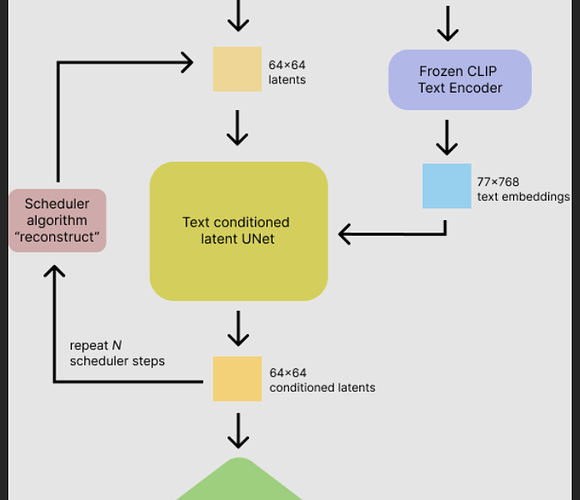
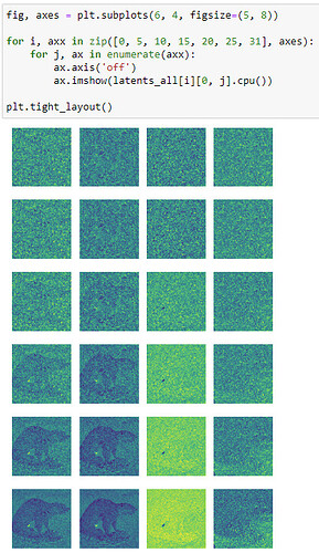
I thought it might be interesting to look at the latents of the otter image from the beginning of the lecture notebook. Here is how they emerge from the noise:

But what was surprising to me was that the latents are just a tiny image?! I mean… why should a compressed representation of an image be a tiny image?

But now I am thinking it probably has to do with how VAE blows up the image! If it uses Convolutions it sort of makes sense (maybe) that pixel intensities should be representative of what they are in the enlarged image?

Anyhow, no clue, need to learn about the VAE bit, but finding this very cool

[jeremy (Jeremy Howard)]

@fredguth

how can I reverse this?
"CLIP embeddings for “A water…” → ??? → "A watercolor of an otter

This is exactly what a diffusion model does! Except it goes from embeddings->image. Something similar to go from embeddings->text might work…

[fredguth]

I was considering this, but I was afraid I was overthinking it and there was an easier way. Still, seems an iteresting idea o try out.

[fredguth]

I have been trying to create a diffusion model that goes from image to text (captioning). As a first step, I thought of creating an image2image pipeline that conditions the unet with the CLIP image embedding, instead of the noisy version of the image as the latent_seed. See: ffc/05-SD-exploration.ipynb at main · fredguth/ffc · GitHub

It took me a while to notice that my understanding of embeddings was wrong. For me, an embedding was the resulting vector that represents the text or the image. But we are also calling the layer that generates that vector as the embedding in the notebook. The conditioning is done by using this last_hidden_layer as a step in the unet, right?

Also noticed that the text and image embeddings in the CLIP model have not the same dimensions, they need to be projected to be compared.

I am stuck with the following problem: unet is expecting an encoder_hidden_states with a 768 dimension, but the image_encoder hidden layer is (257,1024). How can I condition the unet using these image encoder hidden states?

[umar]

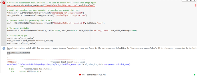
I am trying to run stable diffusion notebook on colab. While running the notebooks I am getting error on this line as shown below:

Can anyone help here?
Do I have to buy colab pro to fix this ?

[jeremy (Jeremy Howard)]

@umar

Do I have to buy colab pro to fix this ?

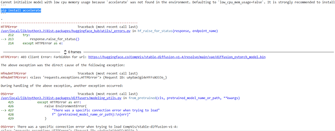
No - read the error carefully. It tells you what you need to run to fix the problem. Let us know what you find!

[umar]

I ran pip install accelerate as suggested here in one cell above this but I am still getting the same error as shown below:

[umar]

I think this is resolved. I had to agree to the terms and conditions of the hugging face website “CompVis/stable-diffusion-v1-4 · Hugging Face” to fix this.

Thanks a Lot

[alexredplanet (Alexander Mars)]

Am a bit late to the party, catching up on the lessons now!

Has anyone ever done local diffusion? i.e. Only changing a small part of the image based on the prompt. Often a change to small part of an image can change its interpretation e.g., a small part of a persons face such as their mouth or eyes can control how their feelings are interpreted.

It would be interesting to take a few pictures of someone with a neutral expression, fine-tune using textual inversion or dreambooth, and see if you can flip the person’s expression with a prompt strongly conditioned by the original image. E.g., Can we make the same person’s face look happy without changing much else in the photo. Feels like it would be an interesting experiment to understand how much these large models are able to understand the key information in the prompt.