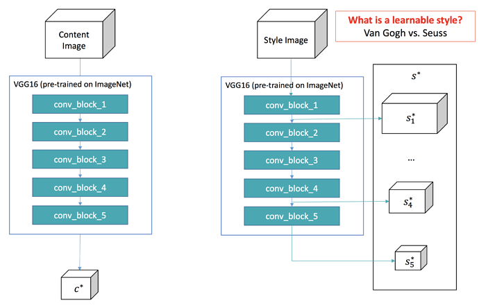
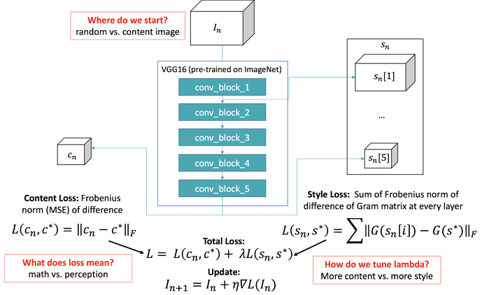
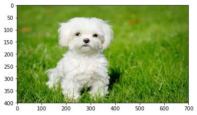
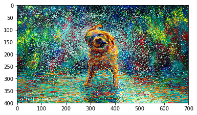
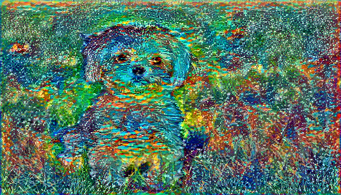
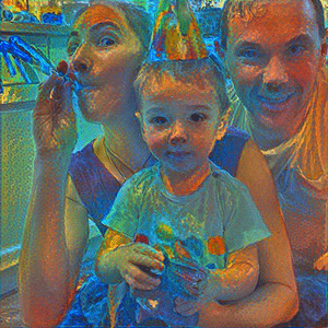
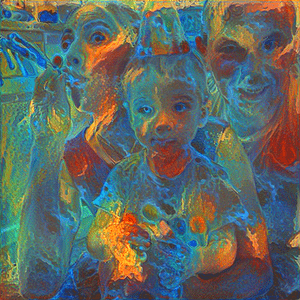
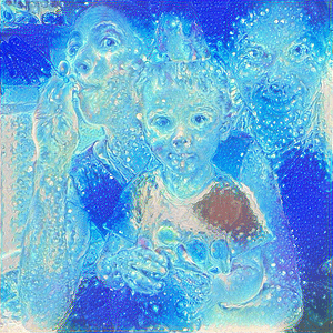
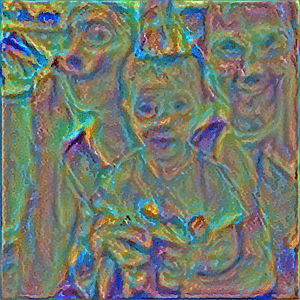
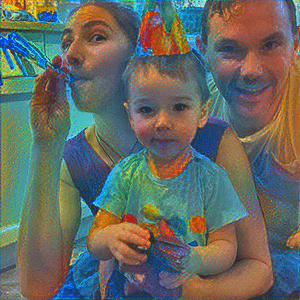
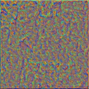
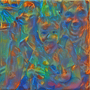
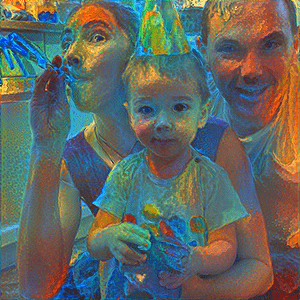
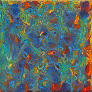
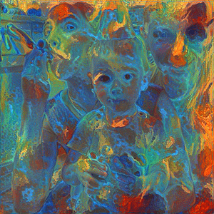
Random aside, I made these block diagrams to help me understand what is going on in the image transfer. Maybe they’re helpful to someone in understanding what is happening better. I also boxed up some of the key questions I have that i’ll be exploring later.
Great post! I’m gonna totally follow this advice 
Saw this paper and wanted to try it out:
The histogram matching thing didn’t work that well for me, but luminance only style transfer worked pretty well.
import os
from scipy.misc import imread, imsave, imresize
from skimage.color import luv2rgb, rgb2luv

def save_luminance(fp, suffix='lum', img_format='png'):
    # save luminance from image, need to do this for style and content
    # then use style transfer on luminance images
    op = '{}_{}.{}'.format(os.path.splitext(fp)[0], suffix, img_format)
    img = imread(fp)
    lum = rgb2luv(img)[...,0]
    imsave(op, lum, format=img_format)

def combine_luminance(a, fp):
    # add uv from original file to output of luminance style transfer
    if a.ndim > 2:
        # grayscale
        a = a.mean(axis=-1)
    assert a.ndim == 2, 'Can only accept 2D or 3D data.'
    img = imresize(imread(fp), (a.shape[0], a.shape[1], 3))
    luv = rgb2luv(img)

    # need to rescale

    mean_a = a.mean()
    std_a = a.std()
    mean_lum = luv[...,0].mean()
    std_lum = luv[...,0].std()
    adjusted_a = (a - mean_a)*(std_lum/std_a) + mean_lum

    luv[...,0] = adjusted_a
    return luv2rgb(luv)
starry night style with luminance only style transfer:
Your theory seems to be right. I tried to turn a fish into an anime fish with Sailor Moon style, but ran into the same poor application of style issue. When you say “start with the original image as the initial condition” to get the better application of Dr. Seuss, what does this mean in implementation?
Is it just me or is this supposed to run on the CPU?
It’s taking a long time for solve_image to run for me. Am I doing something wrong in terms of my setup that doesn’t enable GPU?
On second thought, blurring it a bit may give a better output.
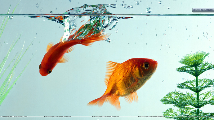
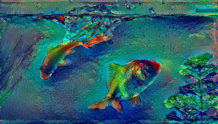
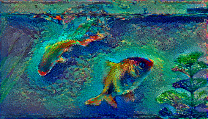
This is what I got for blurring the original image using a Gaussian Filter (size=2).
It has no much obvious difference other than the region between the fishes showing a broken pattern, which I kind of like.
Yeah I think that pattern is much more interesting.
With all these things to tune, it makes me think that there’s room to create a more interactive web app that let’s the user try out lots of knobs and dials to see what looks good. The trick would be so somehow give a very rapid approximate answer so that the user can try lots of ideas quickly…
Can I also point out a questionable statement in the neural-style notebook:
The key difference is our choice of loss function.
There really is no difference in the loss function. It still is MSE.
I think what would be possibly more clear would be , ‘The key difference is transforming our raw convolutional output using a Gram matrix before we use MSE’.
Just an idea. Thanks.
EDIT! After some further thought, saying that “The” key difference implies that there is only one key difference between the prior content of the notebook and what is to follow. It seems that there are specifically 2 key differences – the introduction of the Gram matrix technique and the method of summing 3 sets of activations (i.e. each of the targs).
That’s just one part of the loss function. The full loss function is the layers of computation to create the activations, the gram matrices, etc. Just because MSE is the bit that we’re handing off to keras’ fit function at the end of all that, doesn’t mean that’s the only thing that’s the loss function…
As I’ll show in the next class, the latter is neither necessary not sufficient for style transfer. The use of the gram matrix (or something similar) is the only necessary piece for making the loss function do style transfer.
After significant experimentation I found much more interesting results when I changed the ratio of style loss to content loss by a few orders of magnitude and allowed the style starting point to slowly converge to the content image.
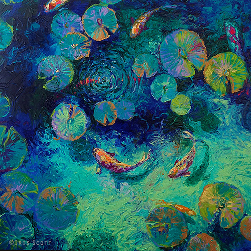
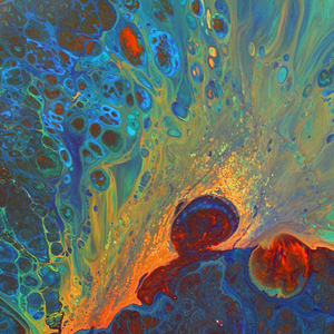
As an example the style layer below (my own artwork):
produces results that I would say match the palette but not the style of the image:
But when I modified the relative weighting of the content to be /2000 rather than /50 the results are (at least to my eye) much more indicative of the original style.
To get the final image I had to train for ~75 epochs, as opposed to the 10 for the first image, and the first few images didn’t really look anything like the content image, but by image 3 or 4 the faces began to emerge.
Here’s my loss function for anyone interested if they want to try it out for themselves:
loss = sum(style_loss(l1[0], l2[0]) for l1,l2 in zip(style_layers, style_targs))
loss += metrics.mse(block4_conv2, content_targ)/1000.
loss += metrics.mse(block3_conv3, second_content_targ)/2000.
I did find that it wasn’t necessary for a number of style images, particularly those that were made up mainly of repeating patterns but for the most styles I consistently got better results with a loss function that focused on style and had a content loss factor that was several orders of magnitude lower than our starting point.
I’ve read another paper that suggests that this ratio could be a parameter of the network, although I’m not sure I understand how that would be possible as my understanding of this space is that we want a fixed loss function and that would change it.
Given that the output depends dramatically on that ratio it would be nice if there were some way of automatically calculating the ratio though.
Here’s another example of the same image for fun:
It’s worth noting that I tried this with much more sparse line drawing style images and the results were terrible, so it could just be that the level of texture and detail dictate the ratio and that could be a reasonable way of calculating it automatically.
Could you explain this bit more?
Sure, i’ll give it a shot… It’s easiest understood when looking at images.
With a content loss to style loss ratio of 1:10 the image generated by the first epoch is:
which already contains a lot of the details and by epoch 10 we have an image that looks like:
If we set the ratio of content to style to 1:100 we have an initial image that looks like our first style image:
and within a few epochs (3 in this case) we begin to see the content details:
and if we continue training for 25 epochs we still end up with an image that converges closer to the content, although it’s a little more interesting and looks like:
If we set our content to style ratio to 1:1000 we have an initial set of images that look nothing like our content image, for example this is epoch 5’s output:
but as we continue training we begin to see the content image begin to appear. Here is epoch 10:
And here is epoch 25:
Training longer (75 epochs) produced the image I posted above.
I found it really interesting how much that ratio impacted the final results.
OK I see what you’re saying I think: set the style/content ratio high, and then train for a larger number of iterations.
Thanks for the explanation.
