Based on my understanding, having a bias for each weight would still be equivalent to having a single value for the entire neuron, since you could just sum all the biases for each pixel and end up with a single value.
Basically, each neuron is wired up to all the input values (i.e. each pixel in the image) and amplified/attenuated by the weight for that input pixel before being added up. We then add up a bias for the entire thing. If we had a bias for each input value (e.g. pixel), we could just total them up to an equivalent single value – does this make sense?
Hey @butchland yeah I think your answer is the right explanation. Thanks, it didn’t occur to me earlier that it all boils down to one bias term effectively.
I’ve made a solid attempt at the full mnist from scratch and learnt a lot.
It looks like its working fine when I define a neural net as a function.
def init_params(size, std=1.0):
  return (torch.randn(size)*std).requires_grad_()

# initialise weights and biases for each of the linear layers
w1 = init_params((28*28,30))
b1 = init_params(30)
w2 = init_params((30,10)) # 10 final activations
b2 = init_params(10) # 10 final activations
params = w1,b1,w2,b2

def simple_net(xb):
    res = xb@w1 + b1
    res = res.max(tensor(0.0))
    res = res@w2 + b2
    return res
In, y =w*x + b, x is just a single input or pixel. You can rewrite this as y = w1x1 + b.
If there are more inputs (e.g. 3), the equation might look like y = w1x1 + w2x2 + w3x3 + b.
You need one weight for each of the inputs or pixels. You only need one bias no matter how many inputs.
In the mnist example, there are 28x28 pixels to start with and therefore we need to initialise and train 28x28 weights and 1 bias for a single linear layer with 1 activation.
The reason for this is that loss.backward actually adds the gradients of loss to any gradients that are currently stored. So, we have to set the current gradients to 0 first:
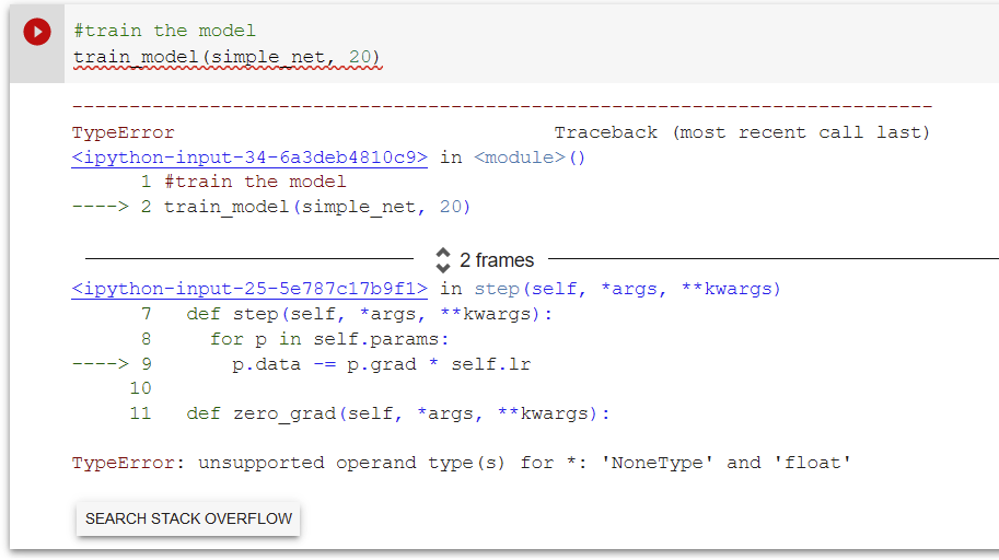
In terms of why is this implemented this way, these are the steps involved in SGD. Stepping the parameters is the final step before we calculate the loss once again or end training.
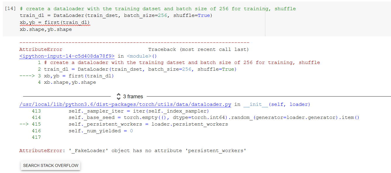
Hi Adi! I wanted to look into your code, but I can’t get it to run without errors, maybe it’s something about the new fastai and PyTorch versions on colab?
Regarding the actual problem, it looks like training is running fine, it’s just the metric that seems off, right? Did you try the out-of-the-box accuracy function?
Thanks for looking into this. Yes, the errors seem to be due to some compatibility issues with fastai and fastcore versions in colab. I get passed these errors when I downgraded fastcore to an older version and similarly with pytorch.
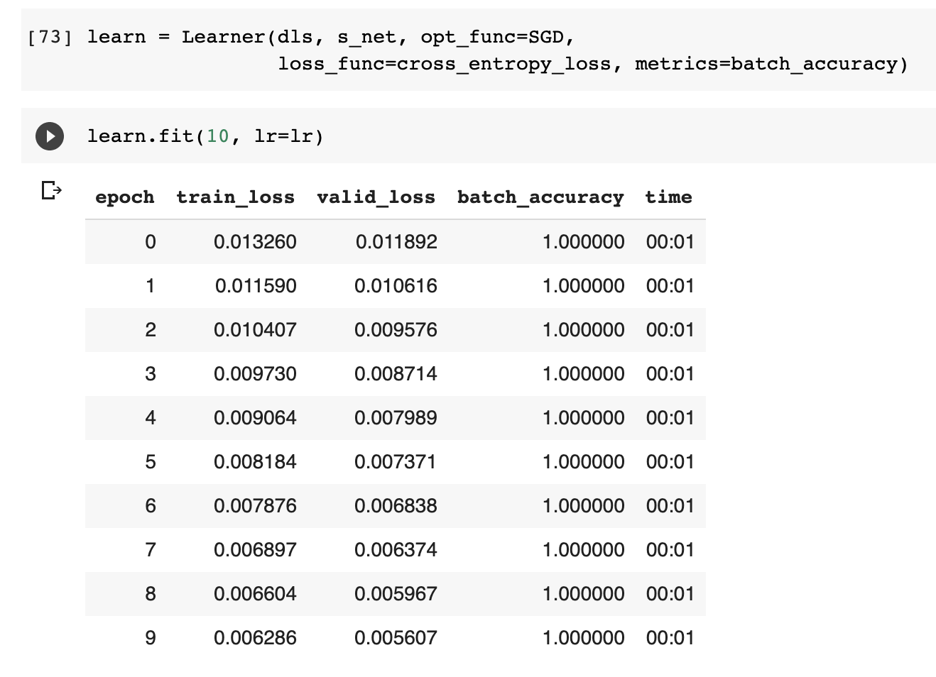
When I built a neural net as a function, the training works fine and the metrics print as expected.
When I try it with nn.Sequential, the training and validation loss decreases (which is great) but the metrics print funny.
I tried the out of the box accuracy metric it still prints 1.00 which is very odd.
My goal is to build the full mnist trainer from scratch and map it to the refactored or convenient version to strengthen my understanding. Really appreciate the help!
Calculate the gradient, which measures for each weight, how changing that weight would change the loss
Step (that is, change) all the weights based on that calculation.
Go back to the step 2, and repeat the process.
Iterate until you decide to stop the training process (for instance, because the model is good enough or you don’t want to wait any longer).
PyTorch provides us with a handy way to calculate the gradient.
We “tag” the initial randomised weights using requires_grad_(). Check out the init_params function in the lesson.
Make the prediction. This is applying our inputs (xb mini batch from the training dataloader) to the model.
Calculate the loss using our loss function -> we define this as mnist_loss in the lesson
Calculate the gradients with the loss.backward() method
We then step the weights by the loss * learning rate
We zero out the gradients because loss.backward actually adds the gradients of the loss to any gradients that are stored. If we don’t take zero our the gradients, the loss for the next epoch will be incorrect.
We repeat training for however many epochs we want. Usually this is until we reach a satisfactory accuracy (using the validation dataloader).
Right, that all makes sense, thank you for clarifying.
I think I’m not asking the question well, let me try it this way.
Since we’re zero-ing out the gradients in step 6, what is the purpose of adding the gradients back into the loss if we don’t zero them out?
I was reading through PyTorch docs but they don’t explain the reasoning behind that functionality or it’s applications. I spent some time googling around but didn’t find any discussions around that either - probably not googling for the right terms though.
Hey Adi, I tried again today but can’t run the notebook without errors. I installed the older versions of the libraries but I can’t run the training loop:
I did find an interesting error though. Check your dataset - all the targets are zero! The error is in the create_xy function, count=0 should not be in the for loop but outside.
That explains why the accuracy was always 1.00 - the model correctly predicted everything being a zero, because that’s what all images were labeled as
Sorry, I didn’t make that clear at all. I’m asking about loss.backwards() specifically. That is, why does <object>.backwards() support adding gradients back in?
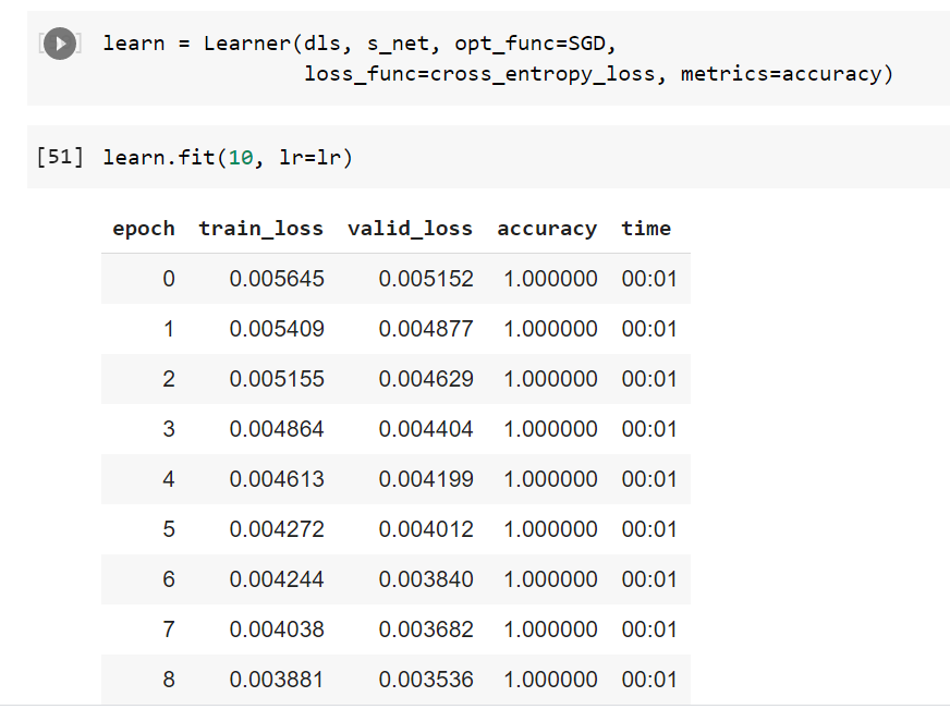
Nice catch @johannesstutz! I updated to code to make sure the labels are correct.
Tested it by indexing into some random values and it appears to be working ok. That’s the good news.
When I ran the rest of the notebook, the accuracy was very low and the training loss did not appear to improve. I think I need to rework some parts of the code and debug.
Hey @misham, I found this StackOverflow answer regarding the default PyTorch behavior of accumulating gradients. Apparently, this behavior is useful for training other architectures, like RNNs. When you don’t need the functionality you just have to manually zero out the gradients.
I have just started learning about RNNs so I can’t give you further details at the moment, maybe that’s just a thing you have to accept as a default
Hey @jellybrain, basically, when you have more than two classes your prediction is not a single number, but every class has its own prediction. In the MNIST example, the model assigns a probability to every digit. The accuracy is then calculated just by picking the class with the highest probability and comparing it to the label. Chapter 5 goes into detail how a loss function for problems with more than 2 classes looks like!
(You can also check out the source code for accuracy, the default fastai accuracy function)