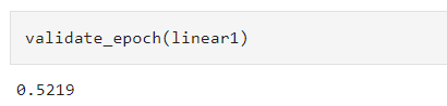
Comparing that code with yours, I can’t see anything that stands out, except perhaps there is a hint that your batch accuracy seems to hit an upper limit at “1”
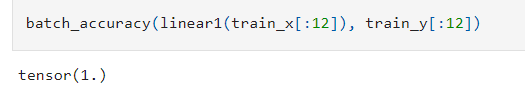
versus the reference notebook starts near the middle.
Comparing that code with yours, I can’t see anything that stands out, except perhaps there is a hint that your batch accuracy seems to hit an upper limit at “1”
versus the reference notebook starts near the middle.
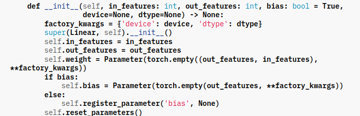
Hi fellow learners. I am going through Chapter 4 in the Fastbook and I got confused by the activation features. It is explicitly stated that the first layer constructs 30 activation features that are passed to the activation function and then to another layer. My question is, how are these 30 activation features computed? I understand that when we specify out_features in torch.nn.Linear as 1, then y is a scalar representing the model’s confidence in what label a particular instance belongs to. However, I do not understand how this is calculated when out_features is greater than 0. I looked into the PyTorch codebase and found out that torch.nn.Linear activates a different set of parameters for every out feature. Is it really the case that when I define 30 output features, the model computes the loss and accompanying gradient on 30 different sets of weights or maybe I am getting it all wrong?
If my understanding is true, then is it the case that these 30 different sets of weights get applied to the same batch from mini-batches per epoch or it is actually randomized?
https://pytorch.org/docs/stable/_modules/torch/nn/modules/linear.html#Linear
Hi all,
I’m working my way through the course and have spent quite a bit of time on chapter 4. After re-reading things a few times, I encountered a question I couldn’t answer myself: I understand we’re calculating gradients to find a minimum and we seem to be doing it with a sort of “trial and error” approach (the whole learning bit).
What I’m trying to figure out is this: Why don’t we “simply” compute the derivative of our loss function? If I remember my high school maths correctly, that’s how you find a minimum (or maximum). What part of our loss function is stopping us from doing that?
I’m really enjoying the course so far and have learnt a ton already. Great teaching style and appreciate making everything available for free.
Cheers
Hey, I was struggling with this myself. I dived into the topic and here is how I understand it now. I’d appreciate if sb could point any flaws in my reasoning.
dL/dw is the gradient of the loss with respect to the model’s parameters, dL/dy is the gradient of the loss with respect to the model’s predicted values y, and dy/dw is the gradient of the model’s predicted values y with respect to the model’s parameters w.*source for point 6,7,8 is Chat-GPT. There is a risk it made some mistakes but I validated it reasoning in this kaggle notebook, where I compare results from PyTorch with symbolic operations using SymPy. The notebook still needs some refactoring but the gradients in PyTorch match the ones calculated as per the explanation I shared. Gradient calculation study | PyTorch vs SymPy | Kaggle
Just finished the book chapter#4 assignment. Oh, gosh, it was pain! Though in the end it felt rewarding.
General thoughts:
It would be nice to have some sort of “on par” bonus requirement for “Complete all the steps in this chapter using the full MNIST datasets. This is a significant project and will take you quite a bit of time to complete! You’ll need to do some of your own research to figure out how to overcome some obstacles you’ll meet on the way.”
Like how many digits should be recognized in valid set.
Book chapter didn’t stress enough on .data.
So when I tried obvious params -= lr * params.grad in reimplemntation task I got an error and had to copy example line by line. (It was mentioned in video with no_grad, but book used .data)
First impression with Fast AI is that it’s way too top-level for its own good and its error handling is pretty much non-existing. Instead of standard exceptions or custom exceptions it just fails. For example if you pass invalid path to ImageDataLoaders, it will complain about None’s.
It also complained something about some tensors being in cuda, some in cpu. How? Why half of tensors end on one device and half of other? I’m not even defining NN or using yet. I even passed device argument. Is 16GB VRAM of Colab’s Tesla T4 not enough for full MNIST? I don’t know, after several days I don’t want to know. I gave up and loaded everything to CPU. Will investigate in future chapters or use other API.
Fast AI’s API is unstable and confusing. At least in notebook. Current version is 2.something.something. If you google for any issue, chances are you find solution which doesn’t work, because it’s for 1.something.something and mentioned solution no longer work.
As an example, I looked how to save/load everything so I can continue training. I found save, export, some tracking callback class, I read about skipping epochs are good knows what else. I tried several combinations, I had all sort of errors from missing dataloaders to mismatching tensor sizes to it simply not working as if weights were reinitialized.
Are these errors caused by my dumb-dumb NN in my brain? Most likely yes.
But when I use KISS torch.save/load_state_dict everything work.
@jeremy I apologize if this is wrong, but I believe there is an error in the fast.ai book, chapter 4 (at least in the Colab version).
This is in the MNIST loss function section. In the section where you are checking accuracy, you say “To decide if an output represents a 3 or a 7, we can just check whether it’s greater than 0.0”, and then you provide the following code to check the accuracy:
corrects = (preds>0.0).float() == train_y
corrects
I believe you meant to check if the prediction probs were greater than 0.5, not greater than 0. Because all (or virtually all) will be > 0
Anyway, I cannot thank you enough for providing this class. I’ll do an intro in the proper place soon, but I just want to briefly say that I’ve done several of the most popular AI courses, and it is almost shocking how much better fast.ai is. I feel like I’m learning SO much faster, and this is the first course that I believe is likely to actually make me into a competent practitioner who can make the products I’m envisioning, without having to spend years learning and then further years at AI companies, learning the foundations. So thank you VERY much ![]()
Hey
Why would you think so? ![]()
0.5 would be the natural threshold if we use a sigmoid function (as in the following chapter) which pushes all predictions between 0 and 1 and lets us interprete the values as probabilites. I tried to give an explanation how the with-sigmoid-threshold 0.5 and the without-sigmoid-thrshold 0.0 are related here.
Hope that helps you make sense of it.
Besides that please have a look at the Forum etiquette regarding @ mentioning people in the forums.
I’m not sure if my answer is technically correct, but I’ll learn something if someone corrects me.
Minimising the loss-function is one step removed from the real goal. The primary goal is to build a sufficiently accurate domain-function mapping inputs to output. The domain-function is the one you would need for you idea to use derivative to find minimum. But this domain-function is the neural network, which changes each iteration, and so is unknown in advance, so cannot be simply-differentiated. Since the loss function is a measure of how good the domain-function is, it also can’t be fully differentiated.
A derivative provides a formula to find the gradient at “any” point. Another way to find another way to find the gradient at a specific point, is to compare the height of two points very close together. This gradient then points towards a better trial point.
Thanks for letting me know about the @ mention rule. Sorry about that.
For something like this, should I just post a message, and if you guys see it you see it? I only used the tag because I thought (incorrectly!) that it was errata that would be useful for you.
As for the threshold - I see what you’re saying. Because the labels are 0 and 1, and because I already knew about the idea of a sigmoidal function, I had assumed that the params were going to optimize to get the output to get closer to 1 if it’s a 3, and closer to 0 if it’s a 7.
But, of course, the parameters are optimizing based on the output of the loss function, and in this case the labels are arbitrary. So, if I’m reasoning correctly, you could basically set the threshold to whatever you want and it will adjust accordingly. And even though the threshold could be anything, 0 is a natural threshold since the params are initialized to center around 0.
My other mistake was in checking how many predictions were less than zero, and when the answer was 3 out of ~12,000, I took that to mean that of course it’s only three, because the output will be between 0 and 1. I figured that since the params were randomly generated, that there should be roughly the same number of 3 predictions vs 7 predictions.
But, firstly, the randomly initialized bias pushes the predictions in a particular direction, and secondly, while the initial parameter values are normally distributed, the pixel values are not. So I tried re-running that little experiment with several different random initializations, and on the second try the results flipped the other way, with basically all the predictions being less than 0.
Anyway, thanks very much for the response. Please let me know if my reasoning here is far off base.
Hey, did you ever find out how to do this without your work-around ? Also facing the same issue
Hello guys, I have tried to reproduce the notebook for Lecture 3 using Google Colab.
The notebook contains my explanations , which can be useful for beginners like me.
Here’s the link: Google Colab
Please let me know if you have any feedback.
Hi there,
I just watched this lecture, and I am pretty sure there is a problem with this piece of code:
for i in range(50):
    loss = quad_mse(abc)
    loss.backward()
    with torch.no_grad(): abc -= abc.grad*0.01
    print(f'step={i}; loss={loss:.2f}')
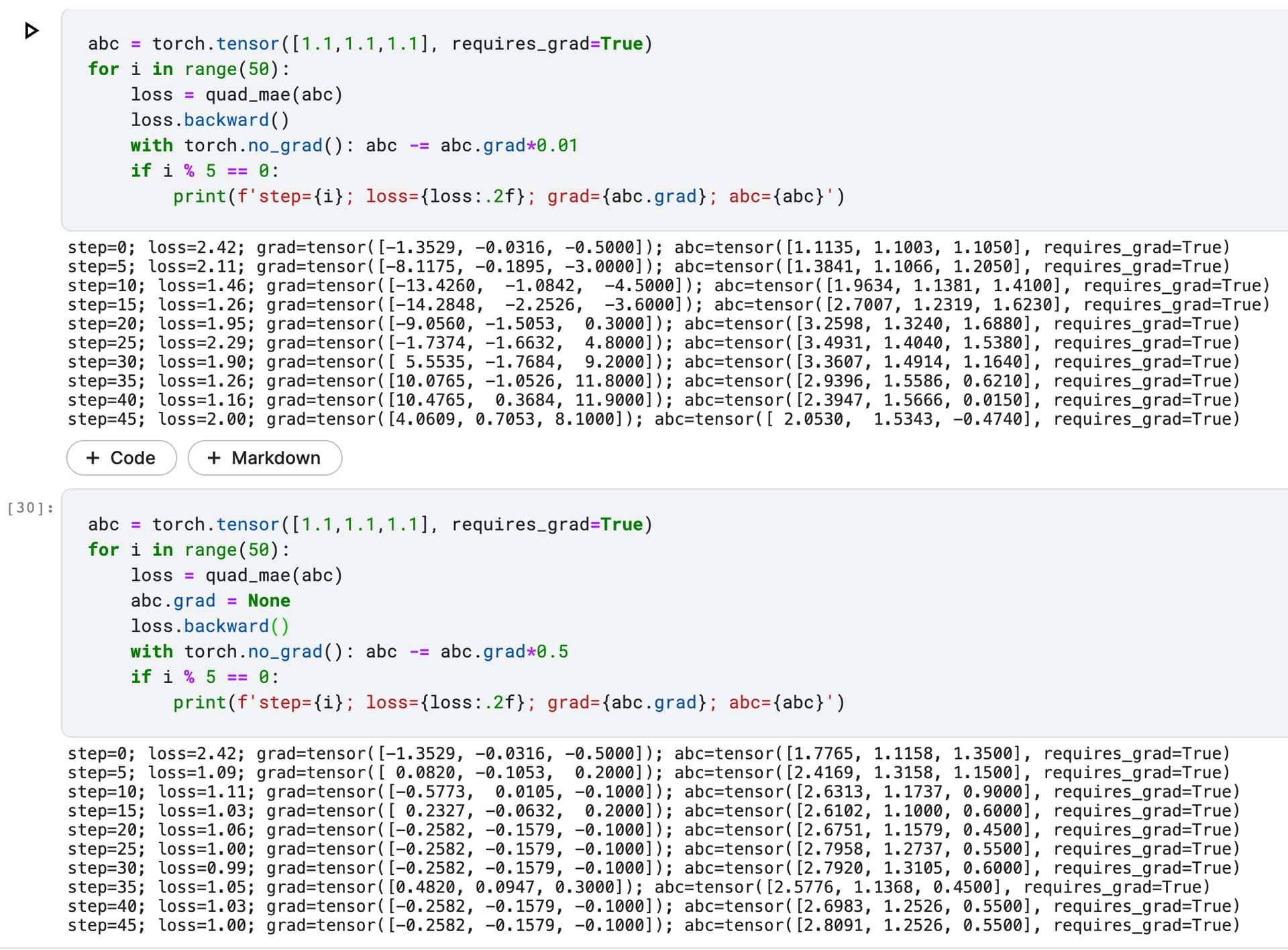
The problem is, is that the grad doesn’t get zeroed which is essential.
I read directly above something about not pinging Jeremy directly, but I am pretty certain this is a mistake. Before each backward pass we should always zero the gradient to flush the values from the previous step.
I am not sure but I think zeroing the grads will be necessary only if we have many mini-batches, but here we have only a small loop of 50 iterations, so no need to reset our gradients.
I am not sure but I think zeroing the grads will be necessary only if we have many mini-batches
![]() I actually don’t think so. In this example we indeed don’t do stochastic gradient descent with batches but instead we do “full” gradient descent taking just one step per epoch based on all our training data (all the x’s and y’s). But that doesn’t matter: we still have to zero the gradient between epochs.
I actually don’t think so. In this example we indeed don’t do stochastic gradient descent with batches but instead we do “full” gradient descent taking just one step per epoch based on all our training data (all the x’s and y’s). But that doesn’t matter: we still have to zero the gradient between epochs.
In the below screenshot you can see the loss, gradients and values of abc for (above) without zeroing the gradient and (underneath) zeroing the gradient. You can see that the gradient is accumulating to quite high values for the first and also totally overshoots the loss, this doesn’t happen when you zero the gradient.
I’m running this cell in the train,ipynb notebook:
dls = ImageDataLoaders.from_name_func(‘.’,
get_image_files(path), valid_pct=0.2, seed=42,
label_func=RegexLabeller(pat = r’^([^/]+)_\d+'),
item_tfms=Resize(224))
and getting this assertion error:
Failed to find “re.compile(‘^([^/]+)_\\d+’)” in “pug_130.jpg”
Any feedback on why this is happening?
Can you check your path variable by entering it in a empty cell and running that cell. It seems to be pointed at that single file or at a folder with images. I think. It should be pointed at a folder with folders with category names with images in it.
When I run
path = untar_data(URLs.PETS)/‘images’
in its own cell, it works as expected (as it did in lesson 2).
But when I run the image data loader in its own cell:
dls = ImageDataLoaders.from_name_func(‘.’,
get_image_files(path), valid_pct=0.2, seed=42,
label_func=RegexLabeller(pat = r’^([^/]+)_\d+'),
item_tfms=Resize(224))
It gives me a lengthy Assertion Error starting with:
Input In [5], in <cell line: 1>()
----> 1 dls = ImageDataLoaders.from_name_func(‘.’,
2 get_image_files(path), valid_pct=0.2, seed=42,
3 label_func=RegexLabeller(pat = r’^([^/]+)_\d+'),
4 item_tfms=Resize(224))
File /usr/local/lib/python3.9/dist-packages/fastai/vision/data.py:149, in ImageDataLoaders.from_name_func(cls, path, fnames, label_func, **kwargs)
147 raise ValueError(“label_func couldn’t be lambda function on Windows”)
148 f = using_attr(label_func, ‘name’)
→ 149 return cls.from_path_func(path, fnames, f, **kwargs)
…
And ending with
AssertionError: Failed to find “re.compile(‘^([^/]+)_\\d+’)” in “pug_130.jpg”
The RegexLabeller is the difference between the working notebook in lesson 2 and this one in lesson 3:
label_func=RegexLabeller(pat = r’^([^/]+)_\d+'),
Any suggestions appreciated!
I resolved this question.
I am getting errors in the Paperspace Gradient notebook.
But it works as expected in the Google Colab Jupyter notebook.
Try using a regex online tester like… random pick… https://regex101.com/
Could somebody explain to me why we use SGD when we can get the optimal solution to parameters that optimizes the loss function, as shown with Excel solver? Is it purely because it is much faster, especially probably with more complicated nets? Will SGD always come to roughly the same accuracy as the optimal solution, or is there some possibility it gets “stuck” on some local optimum point? Thanks.