Updating the course website to recommend Gradient Notebooks
TLDR: it might be helpful to update the course website to say that Gradient Notebooks is currently the best platform for running the course
in the lesson video Jeremy says that Gradient Notebooks is currently the best platform for running this course. he says to check the course website for the most recent recommendation. Lesson 1 suggests Kaggle as the first option for the platform to use, and the Resources page does the same.
Gradient Notebooks out of capacity error
when I try to create a test notebook in Gradient Notebooks I get the message
We are currently out of capacity for the selected VM type. Try again in a few minutes, or select a different instance.
I am trying to create a Free-GPU machine. Has anyone else had this issue? if it’s a common issue it seems like this is a limitation of using the platform.
update 1 hour later: I am now able to create a notebook!
Tensor notation
Does anyone know why values inside a tensor have a dot after them? E.g. page 154 of the book includes the line
Hello, I’m trying to understand the concept of the universal approximation theorem with regard to rectified linear units.
I have 2 points I wanted to see if anyone could clarify:
The first is, there is an implication in the course and the book that you can approximate any arbitrarily squiggly line to any level of accuracy using enough ReLUs chained together. I created an “n_rectified_linear” function, which basically creates as many ReLUs as you want. After creating one that was around 10, I was able to approximate the general quadratic 3x^2 + 2x + 1 to a high level of accuracy in just a few epochs. However, when I tried approximate something like a sine wave with this set of ReLUs (even increasing their amount), it seems to just settle into a straight line that bifurcates the sine wave down near the middle, then stops optimizing. I realized here that ReLUs can’t actually curve back downward - they can start from high up, move down, and then back up, but can’t go back down. Graphing a quadratic that bends the other direction (-3x^2) shows this - it just remains a straight line because it can’t curve that way.
Next, in the book, we learn that with just 2 linear functions separated by a ReLU, we can approximate any arbitrarily squiggly function. In my mind that seems to contradict the findings in #1 - you would have to chain a whole lot of them together to approximate more complex squigglies. The only way I’ve been able to make this fit in my mind is that, when compared to the simple 1 dimensional quadratic-estimating ReLU, the mnist estimator is using 28x28 different parameters (one for each pixel), which produces a 784 dimension linear function. Thus, we could estimate more complex functions by adding parameters instead of chaining additional ReLUs?
Perhaps I’m overthinking this, but I wonder if someone could help me adjust my perspective?
That reads as if you are only chaining ReLUs but you also need linear layers inbetween. I don’t see why your approach wouldn’t work otherwise, but you could share your code here so we can have a look .
Exactly, you can increase complexity by adding layers (increase the depth) or by adding more nodes per layer (increase the width). I think the wiki article offers a good overview if you’re not scared by the math notation
It’s important to realise that the proofs of the (many) universal approximation theorems only show existance but don’t offer a construction. Meaning that even if we know, that for any “squigly” line there exists a neural net that approximates that line, that doesn’t mean that there is an obvious way or any way at all, to receive that network. In particular it doesn’t mean that gradient descent will produce it!
I found this stackexchange post which offers a bit more explanation and a few links if you want to get in deeper:
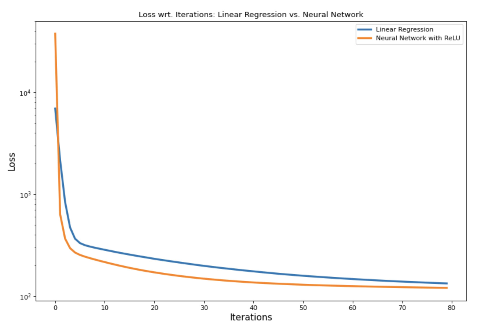
Hello fellow learners, I was trying to understand the excel sheet by following Jeremy’s Lecture 3 video and I realised it’d be a good exercise to implement it in Python. So, ended up writing end-to-end system on it. Wrote everything from scratch – without using any off-the-shelf machine learning framework. I even ended up writing Gradient Decent solver and using it for optimising – all with just NumPy!
I had to figure out and debug a ton of NumPy array dimension issues as well as understand Gradient Decent good enough to implement – which proved to be a very good learning experience.
I also plotted loss vs iterations graph for Linear Regression and Neural Network approach. And as expected got very intuitive results, attaching here the final plot. For given number of iterations, Neural Network does perform better than the linear model.
Seeing this graph after everything was really “aha” moment for me. Thanks to the Jeremy and his amazing teaching method along with active supporting community here!
Here is the the blogpost which implements this in Python. Comments, suggestions, feedback are super welcome!
Thanks a lot of your explanation, your links sent me down a rabbit hole I do not regret!
My realisation with regard to why my chained ReLUs weren’t cooperating was that I needed to adjust for the output space. Chaining ReLUs without adjusting the output space leads to the exact problem I had - you can only encode for a single, upward parabola. However, the fix is quite simply to apply weights and a bias to the output node as well. Since they can be negative, the result can be adjusted in either direction (rather than strictly positive as with plain ReLUs).
I understand now that Jeremy was probably trying to avoid introducing as many concepts as possible (like output node adjustments) while still showing a complete picture of neural networks using ReLUs, while I was diving a bit further in. Regardless, I learned a lot.
For anyone interested in diving a bit deeper into the universal approximation theorem and a slightly different perspective than shown in fastai (at least thus far), cannot recommend this chapter in the Neural Networks and Deep Learning book enough.
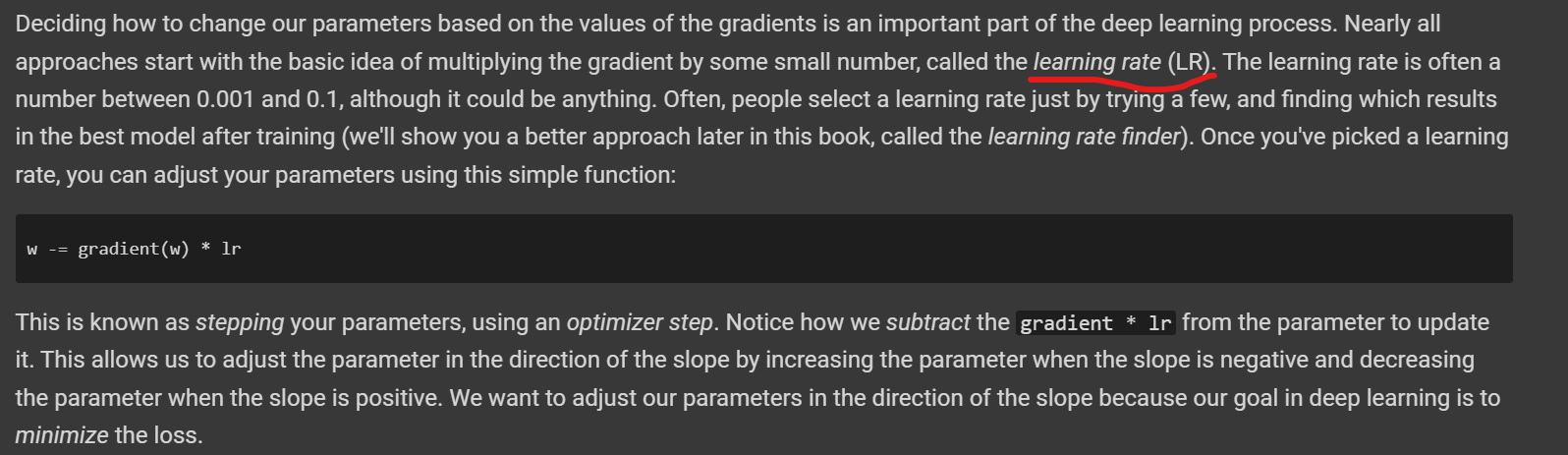
The optimization step is a way to make the loss go down. In order to do this, we subtract the coefficients gradients multiplied by the learning rate from the coefficients. This is explained really well in only about two minutes in this lecture, around the 40 minute mark.
Apologies in advance since I feel this might be a stupid question but I’m having a hard time understanding the formula found at page 146 - Chapter 4: Under the Hood: Training a Digit Classifier. It explains a function that calculates the mean absolute error:
I understand the concept of this function but don’t quite understand the math behind the -1 & -2 values… Would kindly appreciate it if someone could elaborate
Edit:sigh… I spoke a bit too soon since it explains this in detail on the page right after nevermind me, moving along…
I’m trying to do the full process of a deep network on the complete MNIST dataset. But I don’t know how to apply the model to make predictions on the whole folder.
Following the steps on ‘Going deeper’ here to make a model with several layers, I get the data with:
epoch	train_loss	valid_loss	accuracy	time
0	    0.103257	0.064308	0.982143	17:22
But then, we’re not told on how to make predictions on the full ‘testing’ folder. We’ve seen through the chapter of the book a way to understand the step-by-step process by using loops, matrix multiplications, etc. But how do I make predictions on a whole folder like this, using high level and effective coding? I’ve tried to search in other places, but I’m new to fast.ai (and to data science in general), and I’m not capable of solving this.
I’m just looking for a code review and sanity check on my self imposed “homework” project where I took data from bank fraud info and made a NN from the ground up. The accuracy is really really high and it actually kind of worries me.
Thanks so much for this course, it is amazing! Not only for learning about deep learning but even I would say as a demonstration of how to program efficiently and elegantly in python!
One very minor suggestion that would have helped me. When you set the scene for updating params for gradient descent:
def linear1(xb): return xb@weights + bias
Think would be useful to have a small note saying that bias can also be thought of as 1 x wb. Only because this is how it was described in the video when you go through the neural net in excel - there you show how adding an extra column of ones to be multiplied by weights which you solve for is a trick you can do to include an intercept.
I got confused by this because bias on its own looks like this variable is a constant until you see it gets updated directly as per GD in next steps.
Quick question: in the video Jeremy was able to change in the Paperspace Gradient to Jupyter Lab but it seems that I don’t have this icon available in my left panel. Any idea if there was some UI change in the meantime or do I need to somehow activate this functionality (i.e. being able to work in Jupyter Lab instead of Gradient custom view).
@bencoman
Ah, I forgot about that function. It actually came from the book (page) but it’s based on MNIST so it may be incorrect, but my understanding of accuracy isn’t great.