Lesson 3 official topic

Can anyone explain how gradients works here ? As I understand gradient is just a slope of tangent on function’s specific point right?
here we are getting list related to [a,b,c] so how it was calculated?

Q1: are we calculating gradients agains lost function or prediction function
Q2: how we are calculating gradient to see how to adjust a,b,c

A1: We are calculating the gradient against the loss function, which in turn takes the results from the prediction function as well as the actual result (the label)
A2: Pytorch calculates the gradient for us, we just have to enable this by calling .requires_grad_() on the parameters tensor.

I hope this helps. If someone has a better answer / if something in here is incorrect, please let me know as I’m also in the learning process.

1 Like

Yes, pytorch calculates gradients for us.
It is possible to dig into what’s going on mathematically, but it is not very important for learning deep learning.

Hello, I wonder why when we wrote our own train_epoch function we used p.grad to upgrade our parameters:

def train_epoch(model, lr, params):
    for xb, yb in dl:
        calc_grad(xb, yb, model)
        for p in params:
            p.data -= p.grad*lr
            p.grad.zero_()

But when we wrote our optimizer we used p.grad.data:


class BasicOptim:
    def __init__(self,params,lr): self.params,self.lr = list(params),lr

    def step(self, *args, **kwargs):
        for p in self.params: p.data -= p.grad.data * self.lr

    def zero_grad(self, *args, **kwargs):
        for p in self.params: p.grad = None
     

Q1: Is there any difference between those two?

Q2: Also why do we use p.grad = None and not p.grad.zero_()?

@Kamui there are often multiple ways to achieve the same thing. And in your example both ways do exactly the same thing!

1 Like

Thank you!

I’m loving this course but have gotten a little confused on a specific line from the Fastbook chapter 4 (which is associated with lesson 3): Google Colab.

Specifically this: “To decide if an output represents a 3 or a 7, we can just check whether it’s greater than 0.0.”

I don’t see any explanation leading up to this part as to why 0 is the right threshold for distinguishing between 3s and 7s. Given that a 3 is labeled as 1 and 7 is labeled as 0, shouldn’t the threshold be 0.5?

Hi @jaypinho,

Yes, I also think this is somewhat confusing. As far as I am concerned: in this case, it actually doesn’t really matter whether we take a threshold of 0.0 or 0.5 or any value for that matter.

In this case we are just applying one single linear transformation to our input which results in one single number for our output (per image). By setting the threshold at zero, we want the linear layer to be filled with values that result in a value larger than 0 for images with label 3, and result in a value smaller than 0 for images with label 7.

Especially since there is a bias term in the linear layer, the network could also easily learn that it should use a threshold of 0, 0.5 or even 1000.

I hope this helps.

2 Likes

Thank you!

[Sorry if this was a little long-winded, but I spent a while thinking it through, and thought it might be helpful for someone.]

I had the same question and wasn’t entirely satisfied with previous answers - because the sentence ‘To decide if an output represents a 3 or a 7, we can just check whether it’s greater than 0.0’ appears twice in chapter 4’ and I think the answer is different each time.

The first time, this number is arbitrary:

We haven’t introduced a loss function yet, we just have a model (linear1) that takes in load of images as a tensor, and outputs a tensor containing a ‘prediction’ for each image. At this point these predictions are simply numbers from anywhere on the real number line. But we want a way to make these numbers reflect one of two categories - a 3 or a 7. So we can pick an arbitrary point, and say anything above it is a 3, and anything below is a 7 or vice versa.

Note that this is before any learning has been done - the parameters of the model have been initialised randomly, so we are not losing any information by picking an arbitrary dividing line. The statement

corrects = (preds>[arbitrary]).float() == train_y

is not comparing the prediction directly with the target 1 or 0. It is comparing the statement (prediction greater than [arbitraryvalue]) which can be evaluated as True (1) or False (0) with the target 1 or 0. As long as we kept the metric the same throughout the learning process, we could keep tweaking the model to make it more accurate, and (ideally) it would eventually be a model that predicted a number greater than [arbitraryvalue] for 3s and lower for 7s.

However, the second time it appears, 0.0 is not arbitrary, as we have already defined mnist_loss. Within mnist_loss there is a sigmoid function:

def mnist_loss(predictions, targets):
    predictions = predictions.sigmoid()
    return torch.where(targets==1, 1-predictions, predictions).mean()

Now, the loss and the metric aren’t the same thing exactly, but they should represent roughly the same aim - there’s no point in training something to do one thing, and then checking it on a completely different thing. In this case, mnist_loss is low for a given image when the sigmoid of the prediction is close to 1 for a 3 and close to 0 for a 7. Given that a sigmoid curve continuously increases and crosses 0.5 at x=0, this means a model with low loss gives very positive predictions for 3s and very negative predictions for 7s, and the human way of interpreting it is any prediction above 0 is a 3 and any below 0 is a 7. The batch accuracy is the proportion of predictions in a batch that were above 0 for 3s and below 0s for 7s.
3 Likes

Yep, fully agree. In the second case (mnist_loss) we apply a sigmoid to the outputs, so there we should most definitely use a threshold of 0.5 (and not something arbitrary).

1 Like

Hi.

Just wondering if anyone has run into the below error after running the train.ipynb, saving the model, running the app.ipynb file. Im running in colab. The error happens on the the line: learn.predict(im)

/usr/local/lib/python3.9/dist-packages/PIL/Image.py in getattr(self, name)
544 )
545 return self._category
→ 546 raise AttributeError(name)
547
548 @property

AttributeError: read

I have also tried running using the existing saved model but get the error below. If i try duplicate the huggingspace space, i also get this error.

File “/home/user/.local/lib/python3.8/site-packages/torch/nn/modules/module.py”, line 1185, in getattr raise AttributeError(“‘{}’ object has no attribute ‘{}’”.format( AttributeError: ‘LayerNorm2d’ object has no attribute

Thanks,
Ross

I’m stuck on this same question!

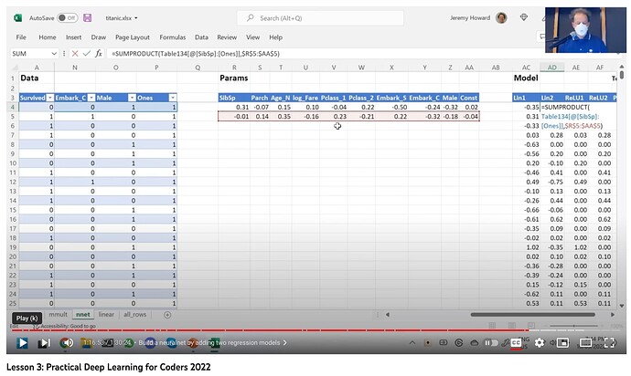
To elaborate, here’s the screenshot I think @yeldarb and I are actually referring to:

These are the two “layers,” and yet both of those rows of coefficients are being multiplied by the independent variable values (e.g. age, gender, etc.). In other words, the order of events seems to be:

  1. Multiple each independent variable by its corresponding weight in the first hidden layer (the first row of randomly-initiated parameters).
  2. Sum up those products.
  3. Calculate the ReLU for that sum (i.e. if it’s under 0, make it 0).
  4. Repeat steps 1-3 for the second hidden layer (the second row of randomly-initiated parameters).
  5. Add those ReLUs together to come up with your prediction.

What confuses me is that this means hidden layer 1 and hidden layer 2 have no real interaction (other than being added together in the final step). In other words, layer 2 isn’t being influenced in any way by the outputs of layer 1 – but I thought the point of neural networks is that each layer influences the one after it, such that the final layer represents the cumulative incremental impact of each of those layers. Is this wrong?

EDIT: One more thought: maybe what’s actually happening here is that those 2 sets of coefficients are not separate layers but are simply 2 separate neurons in the same layer. Then, if you were to create another layer on top of that one, it would use those 2 neurons as inputs to that second layer. This explanation seems to be closer to my understanding of a neural network. (It also seems to align with the description here.)

If this is the case, though, it’s not clear why the 2 neurons in the layer would be added together. Is that always what you have to do to get to a single (Boolean) output layer?

1 Like

You are spot on with this, it indeed mimicks a 1 layer neural network with 2 neurons. On your second observation you are also spot on, generally we would add a second layer of shape (2,1) to get to the final prediction (possibly followed by a sigmoid to get the predictions between 0 and 1 which would match our use case).

But I guess Jeremy is doing it with a simple sum to keep things simple. And the sum would kind of be a second layer of shape (2,1) where the weights are both 1, and no bias term is included.

Hope this helps

1 Like

What version of Fastai are you running? try updating to 2.7.12 - (released on Mar 29th).

Thank you so much for confirming! Wanted to make sure I wasn’t losing my mind. :slight_smile:

1 Like

Hi Allen.

Thanks so much, I re-ran !pip install fastai in colab and the output says: requirement already satisfied: fastai in /usr/local/lib/python3.9/dist-packages (2.7.12).

I re-ran the app.pynb and and its now working perfectly thankfully!
Cheers for all your assistance,

Thanks,
Ross

1 Like

Lesson 3 just blew my mind looking at NN in a bare way!

Around 38 minutes 40 seconds into the lecture, Jeremy shows us calling backward() on the loss function (loss.backward()) computes the gradient for the input (abc.grad). This is confusing to me probably because I have not watched the lecture on backpropagation yet. How come calling backward on loss function gives the gradient for its input parameters? Jeremy later explains that the values in abc.grad are the slopes of the loss function with respect to the three parameters. Does this mean that after calling loss.backward(), the gradients are computed with respect to the input params and then they are saved as gradients of the params (abc in this case)? I would have thought saving the gradients as loss.grad would make more sense.

1 Like

first jeremy create a variable abc

abc = torch.tensor([1.5,1.5,1.5])
abc.requires_grad_() # this tells pytorch that we want to keep track of the gradients of abc

then he computes the loss (quad_mse) of abc

loss = quad_mse(abc)

now when we call backward() on the loss function, we get the gradients for all 3 components of abc (because abc is a tensor with 3 elements)

So loss.backward() gives the derivative of the loss with regard to each one of those 3 elements and stores that in abc.grad.

In order to get a more complete understanding I highly recommend this video by Andrej Karpathy, I can confidently guarantee that once you watch it you will have a very good understanding of gradient descent and backpropagation, it is really worth your time.

1 Like