Applying part 2 to tabular data

[yonatan365 (Yonatan)]

Hi all,

this course has been terrific for me so far since it allows me to understand the inner workings of the fastai’s library and use them for my needs, and in particular, tabular data. In this topic I will present my progress on transforming what we learned to a tabular dataset, namely the dataset from Otto Kaggle competition.

I know about the tabular options fastai provides, but I’d much rather know how to implement stuff on my own. This is for several reasons:

1. More often than not, I need some special customization to the data handling. Images data are mostly similar in shape, but tabular data is very heterogeneous, and each dataset requires tweakings of its own.
2. I’d really like to be able to try the ideas presented here (initialization, custom layers, etc) on my favorite datasets
3. I have several specialized architectures I am developing (mainly related to autoencoders), and I want to benefit from the amazing research tools that were given so far in this course (callbacks, layer statistics, metrics, etc.) while studying them.
4. In the spirit of this course, doing it will force me to use the tools and recreate them for my needs, which to my feeling will be the best way to learn.

And why the Otto dataset?
no strong reason here. Its advantages are that its relatively simple (all features are similar in distribution), has moderate amount of samples (not too long to train, but not tiny), is well rated being a Kaggle competition and I have lots of experience with it…

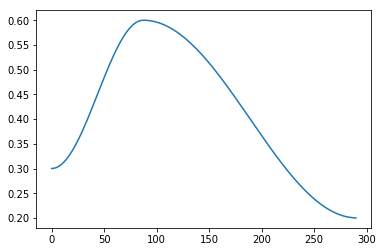
Also, normalization of this dataset is not a trivial issue and I hope the init research on it will provide some new insights.

I’ll use this topic as a kind of a diary for my progress, and I also invite anyone who has similar interests, i.e. trying what we learn on tabular data, to post here as well what she’s doing!

---

I decided to start from notebook #5, and see how it goes from there. The first thing to do is to load Otto dataset, instead of loading MNIST. I override the get_data() function with my own version (after downloading the dataset from Kaggle):

def get_data(valid_pct=0.2):
    import pandas as pd
    df = pd.read_csv('../../../data/otto/train.csv')
    target_name = 'target'
    df[target_name] = df[target_name].astype('category').cat.codes # replace string labels with ints.
    df = df.drop('id',1)
    valid_mask = np.random.rand(len(df)) < valid_pct
    x_train = df.iloc[~valid_mask].drop(target_name,1).values.astype(np.float32)
    y_train = df.iloc[~valid_mask][target_name].values.astype(np.long)
    x_valid = df.iloc[valid_mask].drop(target_name,1).values.astype(np.float32)
    y_valid = df.iloc[valid_mask][target_name].values.astype(np.long)
    return x_train, y_train, x_valid, y_valid

Now I try to continue with the rest of the notebook. We defined in NB#4 the get_model function which returns a pytorch sequential object:
nn.Sequential(nn.Linear(m,nh), nn.ReLU(), nn.Linear(nh,data.c))
Lets look at the model by typing learn.model:

  (0): Linear(in_features=93, out_features=50, bias=True)
  (1): ReLU()
  (2): Linear(in_features=50, out_features=9, bias=True)
)

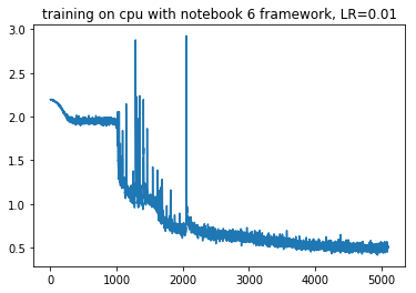
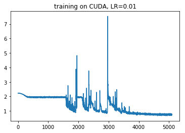
which looks fine for a starting model. Fitting for 20 epochs (LR=0.01) gives:

train: [0.50778127929156, tensor(0.7997)]
valid: [0.5754367667622667, tensor(0.7828)]

It’s not amazing but also not bad. The Kaggle winners got logloss ~ 0.38 and accuracy of above 83% so we still have room for improvement (which is good for our research!). After doing that I noticed I forgot to normalize the data! I do it with:

train_mean,train_std = x_train.mean(),x_train.std()
x_train = normalize(x_train, train_mean, train_std)
x_valid = normalize(x_valid, train_mean, train_std)

and now the results of the same fit are:

train: [0.5099700296131825, tensor(0.8005)]
valid: [0.5568894527170857, tensor(0.7817)]

which is slightly better.

---

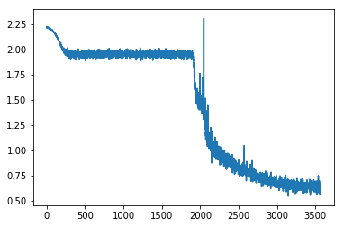
LR Scheduler:
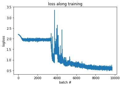
I created the following scheduler

and fitting with that gives

train: [0.5130191078997147, tensor(0.8015)]
valid: [0.5479801731690297, tensor(0.7850)]

Which starts learning slower, as expected, and maybe improves the log-loss in a tiny bit more.

What else can we do? How about initialization?
Embarrassingly, I’m actually not sure what is the initialization I’m using here.
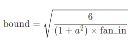
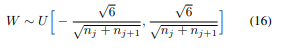
We define the model layers using pytorch linear layer module. We do not provide any arguments there, so the parameters are probably initialized with default. checking the pytorch source for the Linear class, I find it is initialized with:
init.kaiming_uniform_(self.weight, a=math.sqrt(5)) which has the dreaded sqrt(5) Jeremy was referring to, but as we saw in lesson 9, in the uniform case it is actually correct to have it, or is it? in pytorch docs it says that a is the slope of the leaky relu, but we use normal ReLU, so shouldn’t a be 0? how can we try it now to see what is better?

I think i’ll stop here, because this post is starting to be gigantic. I’ll continue in a new post under this topic.

[yonatan365 (Yonatan)]

Here I continue my adventures… and now initialization. Since we are using pytorch to create the layers, I have to somehow be able to get statistics for the mean and std of each layer weights.

I can access each layer through the model object which contains all the layers.
This code gives me the means and stds of the result of applying layer 1 to the train data:

def print_stats(t):
    print(f'mean: {t.mean()}, std: {t.std()}')

l1 = learn.model[0](torch.from_numpy(x_train))
print_stats(l1)

and results in

mean: 0.04519622400403023, std: 1.4511010646820068

and

l2 = learn.model[2](learn.model[1](l1))
print_stats(l2)

which results in

mean: 0.0937328115105629, std: 0.6294490098953247

repeating the above several times for different random inits shows the mean is fluctuating around 0 and the std is quite stable on the above values. Also interesting to note that in this case the ReLU did not cause a significant increase in the mean. Maybe its related to the distribution of the values of the Otto features, which has a long tail to the right like in this example of feature #4:

That really deserves a research of its own, namely, how the distribution of the input data affects the magic number for init. In tabular data one regularly sees a variety of distributions, and I think that it might not be possible to have one good “magic number” and this number needs to be derived for each dataset separately.

I take a moment to apologize that my code and writing is not nearly as neat and clean as the experiments Jeremy shows us, but on the other hand i’m depicting here the real progress of a student in the course, not an edited version so I can allow myself to keep it this way for now.

So, will initializing to unit std improve our results? I guess not really, since our net now is so shallow. It only has 2 layers, so we won’t really suffer from the consequences of std not close to 1.
Lets check…

I need to change the model weights in order to do that. Its not so straight forward (unless I’m missing something here!). The way I found to do it is kind of hacky. Suppose I want to put 0’s in all of layer 1 weights… I do this :

sd = learn.model.state_dict()
sd['0.weight'] = torch.zeros_like(sd['0.weight'])
learn.model.load_state_dict(sd)

somehow it didn’t work in a more straight forward manner.

So now i’ll scale the weights of each of the 2 layers by the necessary number so the stds will be 1. I do it in the dumbest possible way, by reinitializing the model and running the following code while modifying the 2 magic numbers until the stds are around 1:

sd = learn.model.state_dict()
sd['0.weight'] = sd['0.weight'] * 1.7
learn.model.load_state_dict(sd)
l1 = learn.model[0](torch.from_numpy(x_train))
print_stats(l1)
sd = learn.model.state_dict()
sd['2.weight'] = sd['2.weight'] * 2.6
learn.model.load_state_dict(sd)
l2 = learn.model[2](learn.model[1](l1))
print_stats(l2)

and with the numbers above I get

mean: -0.018672337755560875, std: 0.9939473271369934 # layer 1
mean: -0.02162681706249714, std: 1.0620250701904297 # layer 2

which is OK for now. lets see if it has any effect on training. After 20 epochs, with the LR scheduler as before, I get

train: [0.4801070149821605, tensor(0.8119)]
valid: [0.5478276041242155, tensor(0.7911)]

not dramatically different, as I expected, probably because its only on 2 layers. For more layers, I will have to find a better way of doing the “dumb” iterative process I showed. Since now very deep net is not my major concern, I’ll keep this (interesting!) research for later.

wow, again it comes out pretty long, so i’ll cut here and continue in the next post.

[jeremy (Jeremy Howard)]

which has the dreaded sqrt(5) Jeremy was referring to, but as we saw in lesson 9, in the uniform case it is actually correct to have it, or is it?

Not not correct. Uniform is sqrt(3) not sqrt(5). Also, kaiming_uniform already has the sqrt(3).

[jeremy (Jeremy Howard)]

After doing that I noticed I forgot to normalize the data!

You should normalize per-column, not a single normalization for whole file. (Like in color images we normalize per-channel).

[yonatan365 (Yonatan)]

Oops! Thanks!

I changed the normalization line to account for each feature:

train_mean,train_std = x_train.mean(0),x_train.std(0)
x_train = normalize(x_train, train_mean, train_std)
x_valid = normalize(x_valid, train_mean, train_std)

and after the initial simple fit I get

train: [0.49253924312484787, tensor(0.8086)]
valid: [0.5640987812002785, tensor(0.7798)]

and with scheduler and magic init numbers from the previous post I get

train: [0.4914911436785106, tensor(0.8089)]
valid: [0.5568091733169253, tensor(0.7831)]

Which seems to be slightly worse(!), probably due to random variations. I guess that in this case the correction to the norm does not make a difference because features have similar means and stds anyhow. But I’m going to keep the corrected norm because, well, because it makes more sense.

[yonatan365 (Yonatan)]

Not not correct. Uniform is sqrt(3) not sqrt(5). Also, kaiming_uniform already has the sqrt(3).

Thanks Jeremy,

here I was still a bit puzzled. I’ll try to explain:

As I wrote above, I tried to follow the docs to see what happens to the weights when they are initialized in pytorch’s Linear module. The module’s init calls a reset_parameters function which calls:

init.kaiming_uniform_(self.weight, a=math.sqrt(5))

so reset_parameters is called everytime I initialize a linear layer with these arguments. The gain of sqrt(5) is not coming from the kaiming_uniform function itself, but is being sent as an argument to it!

Now I go deeper to the kaiming_uniform_ function, its definition is:

def kaiming_uniform_(tensor, a=0, mode='fan_in', nonlinearity='leaky_relu')

which actually assumes a leaky relu as default. So in this process I learn that I cannot define any nonlinearity when declaring a linear layer, and it always assumes a leaky relu.

So what init do we finally get?
following in the kaiming_uniform_ function, there is a line to calculate the gain,

gain = calculate_gain(nonlinearity, a)

which in our case will be called with
nonlinearity='leaky_relu' (the default argument in the kaiming_uniform_ function)
and
a=sqrt(5) (the argument we passed to the function).
and return

return math.sqrt(2.0 / (1 + negative_slope ** 2))

which magically turns out to be sqrt(3)! which is the correct number (or is it? see later) but a strange way to get to it…
so finally we get this

std = gain / math.sqrt(fan)
bound = math.sqrt(3.0) * std  # Calculate uniform bounds from standard deviation
with torch.no_grad():
    return tensor.uniform_(-bound, bound)

which gives a uniform distribution between [ \frac{-3}{\sqrt{fan}}, \frac{3}{\sqrt{fan}} ].
Notice that it is 3 here, not \sqrt{3} because we multiply by \sqrt{3} again. Should it be 3?
In the docs, they have a written formula for the bounds of the uniform distribution in Kaiming uniform normalization:

notice there is no \sqrt{3}, neither 3, here!
for ReLU, a=0 and according to the formula we should have U[-\sqrt{6/n}, \sqrt{6/n}] which is not what we finally get (albeit quite near, accidentally, as \sqrt{6}=2.45).

I also tried to look in the academic papers that were mentioned to get a better answer for that. Skimming Kaiming’s paper I don’t see a reference to uniform distribution, but Xavier’s paper discusses it and claims that the initialization should follow

which halfly resembles the formula in the pytorch docs (different in the fan_in+fan_out), and again we see \sqrt{6}. Maybe with the ReLU there is a factor of 2 which causes the \sqrt{6} to become \sqrt{3} but anyhow that is not what I see we finally get from the function itself.

Hopefully I will find an answer to these inaccuracies/mysteries I stumbled on here. Probably some/all of them are related to my confusion. If you (Jeremy or anyone reading this) can shed some light here, it will be great!

[yonatan365 (Yonatan)]

Continuing the progress on Otto dataset -

I think the next interesting stage here will be to significantly increase the number of layers in the model, and check if it learns anything, and which initialization will induce the best training.

How to do that?
I modify the get_model and create_learner functions in the following way:

def get_model(data, layers, lr=0.01):
    model_layers = []
    for k in range(len(layers)-2):
        model_layers.append(nn.Linear(layers[k], layers[k+1]))
        model_layers.append(nn.ReLU())
    model_layers.append(nn.Linear(layers[-2], layers[-1])) # last layer
    model = nn.Sequential(*model_layers)
    return model, optim.SGD(model.parameters(), lr=lr)

def create_learner(model_func, loss_func, data, layers):
    return Learner(*model_func(data, layers), loss_func, data)

and now I can define a model with 10 hidden layers by

m = x_train.shape[1]
c = y_train.max().item()+1
layers = [m] + [40]*10 + [c]
learn = create_learner(get_model, loss_func, data, layers)

I have a feeling this is not going to work… We can look at the training loss along batches using run.recorder.plot_loss():

yes, that looks bad… I’m surprised it managed to learn something at all. The next reasonable step is to initialize this network properly, but before we do that, i’d like to have the tools for diagnosing the mean and variance of each layer along the training. This tool was only developed on notebook #6 when we learned about hooks. So in order to add this functionality i’m going to “upgrade” my framework to the one in notebook 6.

I transferred the functions I re-wrote to notebook 6, and now I’m using the GPU, and hopefully will be able to use the stats hooks from lesson 10. I checked that the model behaves in a similar way, and yes, the results of training 10 hidden layers are still pretty bad as before.

Moving the model to the GPU was supposed to be smooth but strangely the cuda version didn’t seem to learn at all. I tried to reduce the learning rate (from 0.5 to 0.01) and it did start to learn. However after trying several more times I found that this was apparently a random effect, because later sessions, with LR=0.5, did seem to work on the GPU. It seems like the network is quite unstable and can converge to many different solutions. Probably the learning rate is too high. I reduced the learning rate to 0.01, and now I get the following for the CPU

and the following for CUDA

For now i’ll continue and assume that the differences are due to random initialization (although deep deep inside I still suspect the cuda’s learning is worse than the cpu!).

Ok, now that we got that working, we can continue to the stats hooks. Everything pretty much worked, no trouble here, and here are the means for our 10 layer network along training:

I think its viciously awesome! who would have believed that our “innocent” looking declining loss plot (at least after the spike around 2000)

hides such a crazy numerical behavior?

also, we can see that for the first epochs, most of the layers are “stuck” in some kind of cycle, while some of them are slowly evolving:

and finally, lets zoom on what happens in the moment of change, when the network suddenly begins to learn

interesting… Seems like the network was stuck for a while in a cycle (probably in a local minima of the loss landscape), but it managed to get out of there and improve, while still suffering from crazy fluctuations! I’m sure this can be improved significantly - currently its like searching for a minima while sitting in a shaking roller coaster… The amazing thing for me is that somehow the net manages to balance all these shakings of the individual layers and improve the loss. Poor network

I will continue in the next post…

[KevinB (Kevin Bird)]

These are great, thank you for documenting your journey here. Tabular data is definitely something I’m interested in. I wonder if you looked at the weights if it would have a lot of the activations going to 0 and that’s what happens where it eventually starts moving this is that enough of the activations went to 0 that it is now able to run.

[jeremy (Jeremy Howard)]

Hopefully I will find an answer to these inaccuracies/mysteries I stumbled on here.

It’s a bug - see the google+ discussion image where this is confirmed by Soumith, in the slides I showed during the lesson. So you shouldn’t use the pytorch default init.

[jeremy (Jeremy Howard)]

Be careful that my code for activation plots had a bug - they were including validation set as well. Thanks to a PR that’s now fixed in the notebook.

[whamp (Will)]

Hey just wanted to drop in and say I’m really loving this approach to walking through the notebooks but with tabular data, thank you for posting.

[Even (Even Oldridge)]

These are really amazing plots @yonatan365. I’m doing research into tabular deep learning right now, experimenting with some different architectures, and this provides an amazing way to look at the model.

What it’s reminding me of, and it really seems to support their arguments, is the lottery ticket hypothesis paper and the follow up. The core idea behind the paper is that a small percentage of the weights end up with a good init (win the lottery) and end up training to the best solution.

The pattern above looks to me like someone buying consecutive lottery tickets searching for a winner.

[yonatan365 (Yonatan)]

Before I continue the research, I’d like to thank the people who read and reply and find interest in these posts - its great to feel that other people are also interested in what I write: Thank you for your comments!

Today, following @KevinB’s and @Even’s suggestion I’ll check what actually happens to the weights of the net. After that, I intend to use the empirical approach from the “All you need is a good init” paper, (minus the orthonormal thing), to initialize the 10 layer network in hope that the training will improve. So lets get to business…

---

First of all, following Jeremy’s warning, I wanted to fix the stats function so it will only show information from the training phase. I thought I can do it by myself, but Jeremy said it was fixed in a pull request and I thought it might be a good opportunity to learn how to look at these git things…

In the github site, looking at the notebook 6 file, I saw one pull request and opened it. Under the tab “files changed” I could see exactly the changes I should make to the notebook in order for it to work. I simply changed these lines in my version of the notebook. And yes, yes, I know I’m primitive and the right way to do this is to merge the changes into the code on my server with some git magic, but the reality is that I’ll only have these capabilities in a future version of me.

So after the correction, we lose the strange periodic peaks! these were due to the differences between train and validation data, and did not reflect the intrinsic state of the weights!

I’ll have to show again all the previous graphs, in the corrected version:
loss along time on GPU:

and the “means” stats

and zooming around the point where loss starts dropping again:

The fix got rid of these periodic peaks and the crazy fluctuations of the net (looking back now I really should have been more suspicious towards the perfect periodicity! that’s a lesson i’ll remember). So now things look more reasonable (and less amazing) than the previous buggy version… Still, it seems like there is a small initial learning stage, followed by a long plateau of the loss, followed by some sudden crazy struggles after which the network manages to find the way to reduce the loss to a reasonable amount.

Also, looking at the stds along time I can see that the init is clearly not so good - the stds in the initial phase is smaller for each consecutive layer.

Now, lets get on to what happens with the weights of the network along time. The hypothesis, following the previous results and the comments, is that most of the weights get zeroed along training and only when a tiny fraction of the weights is left the net can actually learn. This hypothesis is in slight contrast to the increasing trend of the means along training so I’m not sure its correct but lets check.

In order to check that, I can use Jeremy’s extended append_stats (with the bug fix, i.e. record only at training) to collect also the data of each layer in a histogram. And why histogram? because the full data is big (each layer here has ~40x40 weights) and the histogram lets us control the amount of bins to hold the data. The signature of the torch histogram function is histc(bins, min, max) and it can only be run on the cpu. histc(40, 0, 10) for example will create 40 bins for the values between 0 and 10.

I made a small change in the function to account also for negative activation sizes, by adding .abs() to the line with the histogram. If the hook occurs after the ReLU, it shouldn’t matter, but checking with a debugger the min value of outp in the append_stats function shows negative values can occur in output.

def append_stats(hook, mod, inp, outp):
    if not hasattr(hook,'stats'): hook.stats = ([],[],[])
    means,stds,hists = hook.stats
    if mod.training:
        means.append(outp.data.mean().cpu())
        stds .append(outp.data.std().cpu())
        hists.append(outp.data.cpu().abs().histc(40,0,10)) 

Then we can use Jeremy’s get_min function:

def get_min(h):
    h1 = torch.stack(h.stats[2]).t().float()
    return h1[:1].sum(0)/h1.sum(0)

which tells us how many of our activations are located in the first bin, i.e., between 0 and 0.25 (size of 1 bin: 10/40 bins). This gives us:

Hmm… interesting. So it seems that most of the activations actually are stuck in a too low value during the long plateau period, and get out of there (i.e. many acts increase in value) when learning finally occurs. This is in contrast to our hypothesis… Also, layers seem to alternate in the amount of change in W, i.e. layer 2 small change, layer 3 big change, layer 4 small change, etc. Very strange - any ideas??

Its kind of arbitrary to choose a range of 0-10 for the acts. It’s possible that all acts in a layer will be very small in absolute value (i.e. in the first bin) but their effect won’t be negligible. We need here a kind of inequality measure, to see how far the higher valued weights are from the lower valued weights. The measure I know for that is called “gini inequality measure”, and can be implemented with numpy as shown here.

But now that re-read what I wrote, I feel that I don’t fully understand the mechanism of the hook yet and there is a mess. I understand that we attach a hook to each forward function in each element of the model. Surprisingly, I almost couldn’t find any information about the pytorch hooks. The pytorch docs say: “The forward hook will be executed when a forward call is executed”. So it will happen before the forward I guess. But are we recording stats now both after the linear layer and after the ReLU? both have a forward method. This is not so good, and will probably account for noise in our output. Maybe I should only register these hooks on the linear layers? or only on the ReLUs?

After some trials with the debugger, I learned important stuff:

1. Currently the hooks are registered for all the modules in the model.
2. I have to select only hooks for the linear or ReLU layers in order to see what interests me.
3. The plots above are again misleading and i’ll have to redo them, because they don’t show the activations after the 10 layers of the net as I thought. They show the activations after the first 5 layers and the first 5 relu’s and maybe that’s the reason for the alternating sizes!

Ok, this is getting too long again. I’ll post this and continue in the next one…

[jeremy (Jeremy Howard)]

So it will happen before the forward I guess.

After the forward. That’s why you’re able to access the outputs in your hook function.

[yonatan365 (Yonatan)]

Oh no, I just figured I lost my 3 page long draft with the next things I discovered. Hrrr… that “saved” flag on the bottom is very misleading!

I’ll try to reproduce what I did:

I fixed the issue of the hooks by changing the Hook and Hooks inits to allow a name to each hook so I can filter them by name. It was done in the following way:

class Hook():
    def __init__(self, m, f, name): 
        self.hook = m.register_forward_hook(partial(f, self))
        self.name = name

class Hooks(ListContainer):
    def __init__(self, ms, f): super().__init__([Hook(m, f, m._get_name()) for m in ms])

now I can filter specific modules in my model to show using:

linear_hooks = [h for h in hooks if h.name=='Linear']
relu_hooks = [h for h in hooks if h.name=='ReLU']

and I can then plot the parts that are interesting for me.

I then moved on to initialization. I ranted a bit about how crazy it is that a respected library such as pytorch contains such a basic problem in the initialization of all its layers, that most of the people don’t really know about (I discussed it in depth in one of the replies above). I think its might be preferable for the users not to have initialization at all than having a wrong one implemented.

So with the default pytorch Kaiming_uniform init of the linear layer I get after the usual 70 epochs a score of

train: [0.5789444006975407, tensor(0.7811, device='cuda:0')]
valid: [0.6379683866943181, tensor(0.7638, device='cuda:0')]

and the stats looks as the following:

the min-bin graphs are here:

and we can see that mostly in the plateau stage layer 1, 9 and 10 are active and the rest are dormant. When significant learning starts the other layers activations start to grow too.

I’ll try the (hopefully) correct Kaiming initialization, i.e. specifying explicitly the kind of nonlinearity (otherwise it assumes leaky_relu). I chose normal init because its in the actual original Kaiming paper:

for l in model:
    if isinstance(l, nn.Sequential):
        init.kaiming_normal_(l[0].weight, nonlinearity='relu')
        l[0].bias.data.zero_()

I get

train: [0.6051937907277019, tensor(0.7751, device='cuda:0')]
valid: [0.649643508282735, tensor(0.7614, device='cuda:0')]

which seems worse! But as I discovered before, the results have strong variations so maybe I can’t really conclude anything from the end results. What I definitely see is that we still have that long “plateau” period where most of the layers are dormant.

I guess both methods, the “correct” and the wrong one, are not really correct at all.
I could have delved deeper and check whether the layers really have std of 1 along the network depth, but now i feel kind of impatient with the analytical methods (Kaiming, Xavier), and more inclined to try the “All you need is a good init” approach which basically say: forget about trying to analytically calculate the right multiplication factor for each layers weight, and just check what is the std and use its inverse as the multiplier to make sure that the layers’ activation std is 1.

Luckily, @simonjhb wrote a clear post and published a notebook about how to implement this initialization! here is the function from the notebook:

def LSUV(model, tol_var=0.01, t_max=100):
    o = x
    for m in model:
        if hasattr(m,'weight'):
            t = 0
            u = m(o)
            while (u.var() - 1).abs() > tol_var and t < t_max:
                t += 1
                m.weight.data = m.weight.data/u.std()
                u = m(o)
            o = u
        else:
            o = m(o)
    return model

Now I really don’t understand why we actually need the loop and iterative process here. Isn’t it correct that when one divides some data by its std one gets std=1 by definition? What am I missing? variation among batches? But anyhow, this function will not update the batch in the inner loop, and after 1 iteration is supposed to have std of exactly 1. Also, what about the non linearity? the activations we want to standardize (std->1) are the ones after the ReLU, because these are the inputs of the next layer, right? I think so, but am not sure. So i’d like to change these 2 things in the LSUV function.

I’m posting so I won’t lose this again and continue in the next post… This feels a bit primitive

[jeremy (Jeremy Howard)]

We’ll be doing LSUV tonight. You’ll find a repo in the course repo

[yonatan365 (Yonatan)]

We’ll be doing LSUV tonight. You’ll find a repo in the course repo

Cool! I’ll probably get answers to my questions

And also thanks so much Jeremy for finding the time to read through my (and 1000’s other people’s) posts and commenting. I’m very grateful for the opportunity to learn in this course and be mentored on a personal level. Its not at all trivial! Thank you!

[gerardo (Gerardo Garcia)]

What are the correct weights for each number?

[yonatan365 (Yonatan)]

What it’s reminding me of, and it really seems to support their arguments, is the lottery ticket hypothesis paper and the follow up. The core idea behind the paper is that a small percentage of the weights end up with a good init (win the lottery) and end up training to the best solution.

thanks for the reference Even, looks like an interesting paper (I just skimmed it).
Pruning seems to me like one of the things that should be exploited more in deep learning problems.
One thing that is a bit disappointing though is that most (my estimate) of the papers in the field measure their performance on MNIST or CIFAR. I didn’t check but I think that the data in these datasets is very nicely distributed (i.e. the pixel values), and most of the tabular data is badly distributed, and I wish more people would make a thorough research on such badly distributed datasets…

I hope that soon we will gain more insight about whether what happens in our case is related or not to the lottery ticket effect they are describing.

[bny6613 (Nick)]

I have also been puzzled by that sqrt(3), in case you still haven’t found the answer, check this thread https://forums.fast.ai/t/lesson-8-readings-xavier-and-kaiming-initialization/41715/36?u=bny6613