All you need is a good init
I found the idea from All you need is a good init by Dmytro Mishkin and Jiri Matas of empirically choosing the weights for the initialisation of your network super appealing.
My impression from reading the initialization portions of the Kaiming He paper (https://arxiv.org/abs/1502.01852), the Glorot and Bengio paper (http://proceedings.mlr.press/v9/glorot10a.html) and the Zhang, Dauphin and Ma paper (https://arxiv.org/abs/1901.09321) is that each paper is correcting previous initialization approaches to correct for changing network architectures. Glorot and Bengio are correcting for deeper architectures, He et al. are correcting for changing non-linearities while Zhang et al. are correcting for residual connections.
Taking the approach that Mishkin and Matas propose in ‘All you need is a good init’ means you need to worry much less about the specifics of your network architecture and so it is much more easily applicable to different architectures.
I decided to give implementing the initialization approach a go - my code is in a notebook here https://gist.github.com/simongrest/52404966f0c46f750a823a44618bb06c
Layer Sequential Unit-Variance Initialization
The main idea in the ‘All you need is a good init’ paper is an algorithm the authors call ‘Layer Sequential Unit-Variance Initialization’ or LSUV. Instead of trying to compute a formula for how to scale weights in terms of the dimensions of particular layers, the algorithm instead takes an empirical approach. You feed a batch of input data through the network layer by layer and adjust the initial weights of each layer until the scale of that layer’s outputs are sufficiently close to 1. Here is some pseudo-code for the algorithm.
for each layer L do:
    Initialize weights of L (WL) with some reasonable starting point
    (see the discussion of the Saxe et al. paper below)
    do:
        increment iteration counter Ti++
        do the forward pass with a mini-batch
        calculate the variance of the output of the layer - Var(L(xb))
        Scale the weights WL by sqrt(Var(L(xb)))
           i.e. WL = WL / sqrt(Var(L(xb)))
    while
        |Var(L(xb)) − 1.0| ≥ some tolerance and the Ti < max iterations
Orthonormal initialization
The authors recommend starting with a random orthogonal initialisation. I’ve written some functionality to do this initialisation using a singular value decomposition. I’ve attempted an explanation of what orthogonality is in this context and why it might be desirable in the notebook I linked to above.
    def reset_parameters(self):
        with torch.no_grad():
            self.weight.normal_(0,1)
            self.bias.zero_()
        W = self.weight.data.view([self.weight.shape[0],-1])
        _, _, Vt = torch.svd(W)
        self.weight.data = torch.Tensor(Vt).view(self.weight.shape)
In the notebook I also briefly talk about what a singular value decomposition is - this is what the torch.svd in the above is doing.
There’s a really nice blogpost https://hjweide.github.io/orthogonal-initialization-in-convolutional-layers that helped me think about orthogonality in the context of convolutions.
Comparing CNN output variance: LSUV vs nn.Conv2d initialization
I’ve run some experiments on the output variance of some CNNs of different depths.
I use a convenience function to create a model with the convolution class I specify and an arbitrary number of convolutional layers at the end.
def get_model(convtype=torch.nn.Conv2d, extra_depth=1):
    model = torch.nn.Sequential(
                convtype(1,8,5,stride=2,padding=2),
                convtype(8,16,3,stride=2,padding=1),
                convtype(16,32,3,stride=2,padding=1),
                *[convtype(32,32,3,stride=2,padding=1)
                   for i in range(extra_depth)]
            )
    return model
In order to see the difference in the output variance between the two convolutional initializations I created and initialized 100 instances of four different model architectures with combinations of shallow (extra_dept=1) and deep(extra_depth=30) and nn.Conv2d and my own OrthInitConv2D initialized using LSUV.
shallow_pytorch_stds    = [get_model()(x).std().item() for i in range(100)]
deep_pytorch_stds       = [get_model(extra_depth=30)(x).std().item()
                                         for i in range(100)]
shallow_orthnormal_stds = [LSUV(get_model(convtype=OrthInitConv2D))(x)
                                             .std().item() for i in range(100)]
deep_orthnormal_stds    = [LSUV(get_model(convtype=OrthInitConv2D, extra_depth=30))(x)
                           .std().item() for i in range(100)]
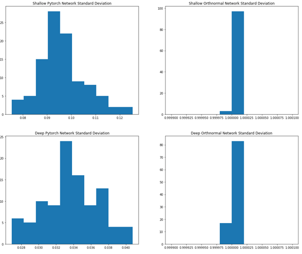
Below is a plot of the histograms of the resulting output variances:
The standard deviations of the shallow PyTorch initialized nn.Conv2d are all quite close to zero, centered around 0.095. For the deeper PyTorch network the standard deviations are even closer to zero - centered around 0.034.
On the other hand the LSUV initialized models both have output standard deviations very closely clustered around 1.
With regards to the stability of training the LSUV initialized shallow network seems to perform similarly to PyTorch initialized shallow network. I need to do some more experimentation with the deeper networks with more appropriate data - I’ll update this post once I have.
Thanks to @ste for helping me think through some of this.
