Applying part 2 to tabular data

Be careful that my code for activation plots had a bug - they were including validation set as well. Thanks to a PR that’s now fixed in the notebook.

1 Like

Hey just wanted to drop in and say I’m really loving this approach to walking through the notebooks but with tabular data, thank you for posting.

2 Likes

These are really amazing plots @yonatan365. I’m doing research into tabular deep learning right now, experimenting with some different architectures, and this provides an amazing way to look at the model.

What it’s reminding me of, and it really seems to support their arguments, is the lottery ticket hypothesis paper and the follow up. The core idea behind the paper is that a small percentage of the weights end up with a good init (win the lottery) and end up training to the best solution.

The pattern above looks to me like someone buying consecutive lottery tickets searching for a winner.

2 Likes

Before I continue the research, I’d like to thank the people who read and reply and find interest in these posts - its great to feel that other people are also interested in what I write: Thank you for your comments!

Today, following @KevinB’s and @Even’s suggestion I’ll check what actually happens to the weights of the net. After that, I intend to use the empirical approach from the “All you need is a good init” paper, (minus the orthonormal thing), to initialize the 10 layer network in hope that the training will improve. So lets get to business…


First of all, following Jeremy’s warning, I wanted to fix the stats function so it will only show information from the training phase. I thought I can do it by myself, but Jeremy said it was fixed in a pull request and I thought it might be a good opportunity to learn how to look at these git things…

In the github site, looking at the notebook 6 file, I saw one pull request and opened it. Under the tab “files changed” I could see exactly the changes I should make to the notebook in order for it to work. I simply changed these lines in my version of the notebook. And yes, yes, I know I’m primitive and the right way to do this is to merge the changes into the code on my server with some git magic, but the reality is that I’ll only have these capabilities in a future version of me.

So after the correction, we lose the strange periodic peaks! these were due to the differences between train and validation data, and did not reflect the intrinsic state of the weights!

I’ll have to show again all the previous graphs, in the corrected version:
loss along time on GPU:
image
and the “means” stats
image
and zooming around the point where loss starts dropping again:
image

The fix got rid of these periodic peaks and the crazy fluctuations of the net (looking back now I really should have been more suspicious towards the perfect periodicity! that’s a lesson i’ll remember). So now things look more reasonable (and less amazing) than the previous buggy version… Still, it seems like there is a small initial learning stage, followed by a long plateau of the loss, followed by some sudden crazy struggles after which the network manages to find the way to reduce the loss to a reasonable amount.

Also, looking at the stds along time I can see that the init is clearly not so good - the stds in the initial phase is smaller for each consecutive layer.
image

Now, lets get on to what happens with the weights of the network along time. The hypothesis, following the previous results and the comments, is that most of the weights get zeroed along training and only when a tiny fraction of the weights is left the net can actually learn. This hypothesis is in slight contrast to the increasing trend of the means along training so I’m not sure its correct but lets check.

In order to check that, I can use Jeremy’s extended append_stats (with the bug fix, i.e. record only at training) to collect also the data of each layer in a histogram. And why histogram? because the full data is big (each layer here has ~40x40 weights) and the histogram lets us control the amount of bins to hold the data. The signature of the torch histogram function is histc(bins, min, max) and it can only be run on the cpu. histc(40, 0, 10) for example will create 40 bins for the values between 0 and 10.

I made a small change in the function to account also for negative activation sizes, by adding .abs() to the line with the histogram. If the hook occurs after the ReLU, it shouldn’t matter, but checking with a debugger the min value of outp in the append_stats function shows negative values can occur in output.

def append_stats(hook, mod, inp, outp):
    if not hasattr(hook,'stats'): hook.stats = ([],[],[])
    means,stds,hists = hook.stats
    if mod.training:
        means.append(outp.data.mean().cpu())
        stds .append(outp.data.std().cpu())
        hists.append(outp.data.cpu().abs().histc(40,0,10)) 

Then we can use Jeremy’s get_min function:

def get_min(h):
    h1 = torch.stack(h.stats[2]).t().float()
    return h1[:1].sum(0)/h1.sum(0)

which tells us how many of our activations are located in the first bin, i.e., between 0 and 0.25 (size of 1 bin: 10/40 bins). This gives us:


Hmm… interesting. So it seems that most of the activations actually are stuck in a too low value during the long plateau period, and get out of there (i.e. many acts increase in value) when learning finally occurs. This is in contrast to our hypothesis… Also, layers seem to alternate in the amount of change in W, i.e. layer 2 small change, layer 3 big change, layer 4 small change, etc. Very strange - any ideas??

Its kind of arbitrary to choose a range of 0-10 for the acts. It’s possible that all acts in a layer will be very small in absolute value (i.e. in the first bin) but their effect won’t be negligible. We need here a kind of inequality measure, to see how far the higher valued weights are from the lower valued weights. The measure I know for that is called “gini inequality measure”, and can be implemented with numpy as shown here.

But now that re-read what I wrote, I feel that I don’t fully understand the mechanism of the hook yet and there is a mess. I understand that we attach a hook to each forward function in each element of the model. Surprisingly, I almost couldn’t find any information about the pytorch hooks. The pytorch docs say: “The forward hook will be executed when a forward call is executed”. So it will happen before the forward I guess. But are we recording stats now both after the linear layer and after the ReLU? both have a forward method. This is not so good, and will probably account for noise in our output. Maybe I should only register these hooks on the linear layers? or only on the ReLUs?

After some trials with the debugger, I learned important stuff:

  1. Currently the hooks are registered for all the modules in the model.
  2. I have to select only hooks for the linear or ReLU layers in order to see what interests me.
  3. The plots above are again misleading and i’ll have to redo them, because they don’t show the activations after the 10 layers of the net as I thought. They show the activations after the first 5 layers and the first 5 relu’s and maybe that’s the reason for the alternating sizes!

Ok, this is getting too long again. I’ll post this and continue in the next one…

5 Likes

After the forward. That’s why you’re able to access the outputs in your hook function.

1 Like

Oh no, I just figured I lost my 3 page long draft with the next things I discovered. Hrrr… that “saved” flag on the bottom is very misleading!

I’ll try to reproduce what I did:

I fixed the issue of the hooks by changing the Hook and Hooks inits to allow a name to each hook so I can filter them by name. It was done in the following way:

class Hook():
    def __init__(self, m, f, name): 
        self.hook = m.register_forward_hook(partial(f, self))
        self.name = name
class Hooks(ListContainer):
    def __init__(self, ms, f): super().__init__([Hook(m, f, m._get_name()) for m in ms])

now I can filter specific modules in my model to show using:

linear_hooks = [h for h in hooks if h.name=='Linear']
relu_hooks = [h for h in hooks if h.name=='ReLU']

and I can then plot the parts that are interesting for me.

I then moved on to initialization. I ranted a bit about how crazy it is that a respected library such as pytorch contains such a basic problem in the initialization of all its layers, that most of the people don’t really know about (I discussed it in depth in one of the replies above). I think its might be preferable for the users not to have initialization at all than having a wrong one implemented.

So with the default pytorch Kaiming_uniform init of the linear layer I get after the usual 70 epochs a score of

train: [0.5789444006975407, tensor(0.7811, device='cuda:0')]
valid: [0.6379683866943181, tensor(0.7638, device='cuda:0')]

and the stats looks as the following:


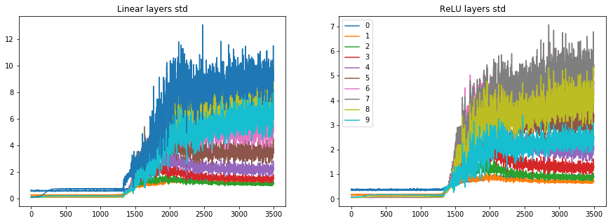
the min-bin graphs are here:


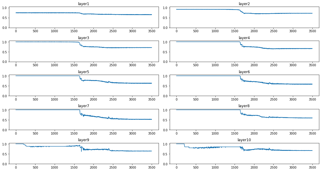
and we can see that mostly in the plateau stage layer 1, 9 and 10 are active and the rest are dormant. When significant learning starts the other layers activations start to grow too.

I’ll try the (hopefully) correct Kaiming initialization, i.e. specifying explicitly the kind of nonlinearity (otherwise it assumes leaky_relu). I chose normal init because its in the actual original Kaiming paper:

for l in model:
    if isinstance(l, nn.Sequential):
        init.kaiming_normal_(l[0].weight, nonlinearity='relu')
        l[0].bias.data.zero_()

I get

train: [0.6051937907277019, tensor(0.7751, device='cuda:0')]
valid: [0.649643508282735, tensor(0.7614, device='cuda:0')]

which seems worse! But as I discovered before, the results have strong variations so maybe I can’t really conclude anything from the end results. What I definitely see is that we still have that long “plateau” period where most of the layers are dormant.

I guess both methods, the “correct” and the wrong one, are not really correct at all.
I could have delved deeper and check whether the layers really have std of 1 along the network depth, but now i feel kind of impatient with the analytical methods (Kaiming, Xavier), and more inclined to try the “All you need is a good init” approach which basically say: forget about trying to analytically calculate the right multiplication factor for each layers weight, and just check what is the std and use its inverse as the multiplier to make sure that the layers’ activation std is 1.

Luckily, @simonjhb wrote a clear post and published a notebook about how to implement this initialization! here is the function from the notebook:

def LSUV(model, tol_var=0.01, t_max=100):
    o = x
    for m in model:
        if hasattr(m,'weight'):
            t = 0
            u = m(o)
            while (u.var() - 1).abs() > tol_var and t < t_max:
                t += 1
                m.weight.data = m.weight.data/u.std()
                u = m(o)
            o = u
        else:
            o = m(o)
    return model

Now I really don’t understand why we actually need the loop and iterative process here. Isn’t it correct that when one divides some data by its std one gets std=1 by definition? What am I missing? variation among batches? But anyhow, this function will not update the batch in the inner loop, and after 1 iteration is supposed to have std of exactly 1. Also, what about the non linearity? the activations we want to standardize (std->1) are the ones after the ReLU, because these are the inputs of the next layer, right? I think so, but am not sure. So i’d like to change these 2 things in the LSUV function.

I’m posting so I won’t lose this again and continue in the next post… This feels a bit primitive :slight_smile:

4 Likes

We’ll be doing LSUV tonight. You’ll find a repo in the course repo :slight_smile:

1 Like

Cool! I’ll probably get answers to my questions :slight_smile:

And also thanks so much Jeremy for finding the time to read through my (and 1000’s other people’s) posts and commenting. I’m very grateful for the opportunity to learn in this course and be mentored on a personal level. Its not at all trivial! Thank you!

2 Likes

What are the correct weights :wink: for each number?

thanks for the reference Even, looks like an interesting paper (I just skimmed it).
Pruning seems to me like one of the things that should be exploited more in deep learning problems.
One thing that is a bit disappointing though is that most (my estimate) of the papers in the field measure their performance on MNIST or CIFAR. I didn’t check but I think that the data in these datasets is very nicely distributed (i.e. the pixel values), and most of the tabular data is badly distributed, and I wish more people would make a thorough research on such badly distributed datasets…

I hope that soon we will gain more insight about whether what happens in our case is related or not to the lottery ticket effect they are describing.

3 Likes

I have also been puzzled by that sqrt(3), in case you still haven’t found the answer, check this thread https://forums.fast.ai/t/lesson-8-readings-xavier-and-kaiming-initialization/41715/36?u=bny6613

Thanks Nick,

I checked the thread and found a nice explanation about why it should be \sqrt{3} but as I explain above the real init (if you use ReLU and the default init) seem to turn out to be 3 and not \sqrt{3} and that’s the real bug in my opinion…

I’m still concerned I got something wrong there - if you or anyone want to double check my reasoning in the reply I wrote above it will be great!

Yeah, you are right, sorry for confusion, i don’t think i can add something else to explain these defaults.

As I said already, it is a bug, and I showed the details of the pytorch team discussing the bug in the lesson slides. Check it out! :slight_smile:

I saw the G+ discussion showed on lesson 9. It focused on the \sqrt{5} and I figured something else (the 3 instead of \sqrt{3} problem even when you state that relu and not leaky_relu is your nonlinearity) but I guess its all just (wrongly implemented) details of the same thing and this Issue that was filed after Jeremy raised it will hopefully improve all of these…

The issue itself don’t explicitly say what the problem is, only that there is a problem. It would be nice if Kaiming He could step in and state his opinion about the correct usage of his init so it won’t be used in a wrong way :slight_smile:

How did you get \sqrt{3} for ‘relu’ nonlinearity? If you pass relu parameter, it gives you the correct gain \sqrt{2} in calculate_gain function

elif nonlinearity == 'relu':
    return math.sqrt(2.0) 

and in this case it works out correctly

std = gain / math.sqrt(fan) 

which gives \sqrt{\frac{2}{fan}} and then in order to calculate the bounds of uniform distribution we multiply by \sqrt{3}.

Thanks Nick, its true about the ReLU, I wrote a mistake above.
I’ll try to say more clearly what I see:

  1. default initialization of linear layers in pytorch always calls the kaiming_uniform with nonlinearity=leaky_relu and a=sqrt(5). I didn’t see a way to use the pytorch initializer with a different non linearity.
  2. the calculate_gain function invoked from kaiming_uniform is returning \sqrt{3} for the arguments: leaky_relu and a=sqrt(5).
  3. after a gain of \sqrt{3} is calculated, the kaiming_uniform returns the gain multiplied again by \sqrt{3} which gives back 3.

so the default init is wrong for ReLU, not because of the \sqrt{5} but because of the extra \sqrt{3} that is multiplied later.

What happens when explicitly stating ReLU for the kaiming_uniform? the calculate_gain will return \sqrt{2} and then it will be multiplied again by the \sqrt{3} so the bounds will be \sqrt{6} which might be correct :slight_smile:

Anyhow, hopefully soon I’ll implement the LSUV with great success and we won’t have to discuss these magic number sqrts anymore!

1 Like

Thanks Yonatan.
For me that multiplication by \sqrt{3} seems correct. Let me just explain my intuition and maybe you can point where i am wrong. So in Kaiming paper they said that for Relu we want to initialize the our weights from distribution with 0 mean and standard deviation \sqrt{\frac{2}{n}}.This is exactly what we get when using nonlinearity = ‘relu’.

std = gain / math.sqrt(fan) #where gain = math.sqrt(2.0)

Next we can sample either from a normal distribution or from a uniform. In case of kaiming_normal function:

std = gain / math.sqrt(fan)
with torch.no_grad():
    return tensor.normal_(0, std)

But in order to sample from the uniform distribution we need to get the bounds. Since the uniform distribution on interval [-bound, bound] has std = \frac{bound}{\sqrt{3}}, to get the bound we have to multiply std by \sqrt{3} which is done in kaiming_uniform function:

std = gain / math.sqrt(fan)
bound = math.sqrt(3.0) * std  # Calculate uniform bounds from standard deviation
with torch.no_grad():
    return tensor.uniform_(-bound, bound)

As i said, i could probably be wrong, just want to make sure i also understand what is going on there.

1 Like

Ok, so that’s the reason! thanks Nick! now I understand it better!

Applying LSUV

In the most recent lesson of the course (11), in a perfect timing for our progress here, Jeremy introduced his version of LSUV implementation. I guess he also decided to skip the orthonormal thing…
His function is the following:

def lsuv_module(m, xb):
    h = Hook(m, append_stat)

    while mdl(xb) is not None and abs(h.mean)  > 1e-3: m.bias -= h.mean
    while mdl(xb) is not None and abs(h.std-1) > 1e-3: m.weight.data /= h.std

    h.remove()
    return h.mean,h.std

Some preliminary remarks about LSUV:

  1. At first I didn’t understand why the iteration is necessary - by definition, anything you divide by its own STD will have an STD=1 after that division. But the reason for the iteration here is that we want the std=1 to apply to activations after the nonlinearity layer. The nonlinearity causes the mean and std to become less predictable and an easy solution here (which i’m not sure is guaranteed to work every time) is to iterate until we are close to what we want.
  2. Jeremy’s code iterates on the first level modules in the model. Our model is currently flat: all the layers, non-linearities, etc. are on the same level. Since, as I wrote above, we are interested in normalizing the activation only after the nonlinearity, (and also to keep our business working with the lesson’s code) I have to aggregate the layers in the model to [Linear, ReLU]. Each pair will then be initialized as one module, resulting in normalizing the activations only after the non linearity.

I made my adaptation of Jeremy’s code, so it will apply the LSUV to our deep FC network. It included importing the data as before, into notebook 7. I also made the following additions/replacements:

class FCLayer(nn.Module):
    def __init__(self, ni, no, sub=0.0, **kwargs):
        super().__init__()
        self.linear = nn.Linear(ni, no)
        self.relu = GeneralRelu(sub=sub, **kwargs)
    
    def forward(self, x): return self.relu(self.linear(x))
    
    @property
    def bias(self): return -self.relu.sub
    @bias.setter
    def bias(self,v): self.relu.sub = -v
    @property
    def weight(self): return self.linear.weight
def get_fc_model(data, layers):
    model_layers = []
    for k in range(len(layers)-2):
        model_layers.append(FCLayer(layers[k], layers[k+1], sub=0))
    model_layers.append(nn.Linear(layers[-2], layers[-1])) # last layer is without ReLU
    return nn.Sequential(*model_layers)
def init_fc_(m, f, nl, a):
    if isinstance(m, nn.Linear):
        f(m.weight, a=0.1, nonlinearity=nl)
        if getattr(m, 'bias', None) is not None: m.bias.data.zero_()
    for l in m.children(): init_cnn_(l, f) # recursively proceed into all children of the model
def init_fc(m, uniform=False, nl='relu', a=0.0):
    f = init.kaiming_uniform_(nonlinearity=nl, a=a) if uniform else init.kaiming_normal_
    init_fc_(m, f, nl, a)
def get_learn_run(layers, data, lr, cbs=None, opt_func=None, uniform=False):
    model = get_fc_model(data, layers)
    init_fc(model, uniform=uniform)
    return get_runner(model, data, lr=lr, cbs=cbs, opt_func=opt_func)

and the actual model initialization happens here (using the same config as before):

sched = combine_scheds([0.3, 0.7], [sched_cos(0.003, 0.6), sched_cos(0.6, 0.002)]) 
cbfs = [Recorder,
        partial(AvgStatsCallback,accuracy),
        partial(ParamScheduler, 'lr', sched)]

layers = [m] + [40]*10 + [c]
opt = optim.SGD(model.parameters(), lr=0.01)

learn,run = get_learn_run(layers, data, 0.01, cbs=cbfs)

this is the loss evolution when training the model in the usual way (with the default Kaiming init):
image
and these are the metrics after 80 epochs:

train: [0.560090118024993, tensor(0.7870)]
valid: [0.6289463995033012, tensor(0.7657)]

The LSUV module just worked (after I made all the changes). Here are the means and stds before the LSUV init:

0.20017094910144806 0.37257224321365356
0.10089337080717087 0.16290006041526794
0.030267242342233658 0.05773892626166344
0.04704240337014198 0.05144619196653366
0.0308739822357893 0.051715634763240814
0.03219463303685188 0.047352347522974014
0.02379254810512066 0.041318196803331375
0.031485360115766525 0.04568878561258316
0.04652426764369011 0.05621001869440079
0.04491248354315758 0.06492853164672852

and after the LSUV:

(0.3296891152858734, 0.9999774694442749)
(0.3093450665473938, 0.9999678134918213)
(0.3306814730167389, 0.9998359680175781)
(0.2864744961261749, 1.0004031658172607)
(0.2594984173774719, 0.9999544024467468)
(0.23850639164447784, 1.0)
(0.20919467508792877, 0.9999997019767761)
(0.2371777594089508, 0.9999346137046814)
(0.16776584088802338, 0.9999942779541016)
(0.17556752264499664, 0.9999728202819824)

A significant improvement. Let’s train it:
image
Wow, still slightly bumpy but much much better. Its faster and more stable (the original init sometimes didn’t converge after 80 epochs). The plateau is gone…

And the final metrics are much better for the training, and less good for validation:

train: [0.3298365177516958, tensor(0.8721)]
valid: [0.6690512438988577, tensor(0.7803)]

According to Jeremy, we have 2 stages in training a model:

  1. overfit.
  2. reduce overfitting.

I didn’t put a good figure for that here, but I can tell you that now (unlike before) the validation dives to around 0.60 before going up again so we managed to pass the first of the two stages: overfit.

Next i’ll try to show more detailed stats of what is going on in each layer, and then I’ll try to reduce the overfitting to improve validation score!

7 Likes