This is a forum wiki thread, so you all can edit this post to add/change/organize info to help make it better! To edit, click on the little pencil icon at the bottom of this post. Here’s a pic of what to look for:
<<< Wiki: Lesson 2 | Wiki: Lesson 4 >>>
Lesson resources
- Lesson video
- Lesson notes from @hiromi
- Jupyter notebook with annotations by Tim Lee
Notes from @melissa.fabros
Techniques for working with “Big Data”
Let’s use Corporación Favorita Grocery Sales Forecasting to practice feature exploration and extraction in large datasets. This is a dataset with over a 100 million rows. How do we process and explore a dataset that we can hardly fit into memory? More importantly how do we define the problem we’re working on if we’re flooded with data.
Defining the problem and the shape of the data
The key thing to define a machine problem is to identify what are the independent and dependent variable in the data. The dependent variable is the thing you’re trying to predict.
In the case of the Favorita Grocery problem, we’re trying to predict how many units, of each kind of product was sold in each store, on each day of a two-week period
The information we have is the how many units, of each kind of product were sold in each store over a four-year period. We see that Corporación Favorita Grocery Sales data consists of several csv files. The data is organized as a relational dataset. There is one central transaction table/csv (in this case, the central table is train.csv) and the other csv files have additional meta data. We’ll need to join the metadata tables around the central one. This data warehousing pattern is called a star schema, which special format of the snowflake schema
Use “Tiny Data” for Initial Exploration :
Take a tiny subsets of the different csvs to start exploring the types of data. We’ll portion off the first 5 lines of data in our train.csv into its own subset.
head -5 train.csv > tiny_subset.csv
Our first exploration is to read in tiny_subset.csv with pandas library. We can use the tiny_subset, to figure out what the datatypes are with pandas before reading in the whole table. tiny_subset.csv lets us explore dataset’s features quickly because we can execute code in seconds instead of minutes. For example, We learn the datatypes for each column in tiny_subset.csv are:
types = {

‘id’ : ‘int64’,

‘item_nbr’  : ‘int32’

‘store_nbr’: ‘int8’

‘unit_sales’: ‘float32’

’onpromotion’: ‘object’

}
From our tiny_subset.csv, we know that we have a ‘dates’ column, so we can tell pandas to parse that column as a date. After our initial exploration, we know what the major data types and features are and can optimize the reading in the whole train file.
df_all = pd.read_csv(‘path-to-/train.csv’, parse_dates = [‘dates’], dtype = types, infer_datetime_format = True}
After our initial processing, the whole train.csv file now can be loaded in 1.48 seconds with very little data tweaking or corrections.
Designing a dev_set or sample set
You can’t do any machine learning until you understand the conditions you’re trying to predict. We’ll a larger dataset than tiny_set to understand what any trends are, and We’ll need to design a development set that runs in 10 second s or less; let’s look at the dates of transaction as data point to anchor the dev_set.
We’re trying to predict sales for a 2-week period and we have four years of data. If you have four years of data, but you only have to have to predict a 2-week period. You can pick the last month of data as a subset for a dev_set. Your goal is to design a subsample data set that will run fast (in 10s vs. 2min).
Isn’t 4 years of data still useful? Isn’t more data better? Yes, you’ll have insight for all four years. We’re not ignoring it, but right now we’re examining the major features of the data. You can explore how long different subsamples takes to run: a month’s worth of data, 2-months, 6-month etc. You can the how long it takes to compare full dataset versus different sized sub-samples to find sample subset that still runs fast and provides enough insight into the data.
data cleaning
’onpromotion’ is read in as a python object, a general purpose python data structure. It runs slowly, but this categories empty values and “na” values. It’s not easy to parse upon upload. After checking your sample, you realize what ‘onpromotion’ data looks like after exploring the category you can fill in the empty values as “False” and then convert the category to boolean values for the whole dataset. You’ll have cleaner data and data in a faster format after fixing the ‘onpromotion’ category. The whole 123-million lines of data can be written to .feather format in 4 seconds.
In Kaggle competitions this means reading the overview and data annotations. With Favorita, we have to convert unit sales to a log of unit sales because sales are expressed in ratios. Also, there will be negative numbers in the unit sales because these represent returned items, and these should be considered as 0 values. We need to represent unit sales as (logarithm of unit sales) + 1, because that’s what Favorita cares about. You’ll want to run all these conversions on the sample sets first because you don’t want to wait 2 minutes to see if the function works or not. Exploring the data also mean taking in account what the client cares about.
Q: Will a transformation of our independent variable affect modeling accuracy?
Such transformations don’t matter for Random Forests. Log of unit sales will still give as accurate a model as to one without the logarithmic transformation.
First exploration steps
After cleaning and optimizing the dataset we’ll read in whole dataset as df_all with pandas, and use df_all.describe(include=’all’) to get summary stats about the data.
Usually in structured datasets, dates and time are very important. You’ll be introducing the evaluation data after you’ve trained the model. You want to make sure that the dates don’t overlap. If anything in the state of the data’s world changes, you’ll want your model to be able to pick up or respond to those changes. For Favorita Grocery competition, the training data dates start in 1/1/2013 until 8/15/2017 and the test data dates start one day later on 8/16/2017 and ends 8/31/2017. After exploring the test.csv, you know that the goal is to predict the next 2 weeks.
Now that you know more about the goal of the prediction, we can use this to inform how we make our sample (aka dev) set. Is randomly picking dates the best way to pick a date range for our sample set or can we do better? Yes! The latest date ranges in dataset would likely be most informative.
If you have trouble thinking about these ideas in the abstract, reframe expression of the problem in physically concrete terms. If you make a bet with a friend predicting how many Coke bottles will be on the shelf tomorrow, you’d go to the store and check the number today instead of ask the owner how many were on the store four years ago.
Jeremy very rarely calls the full dataset for random forest analysis. He only needs as much of the data that will show the types of relationship that are involved. Once you’re comfortable with what’s in the sample, then you can move on.
Manipulating and managing a large dataset:
The need for speed
After reading in our csv data as dataframes, we’ll use feather format to write and read our dataframes to disk. Feather format reads/writes to disk as fast as reading/writing to memory.
We can time our functions with %time in front of any function in your jupyter notebook and can measure how long it takes a function to run. In addition you can run %prun in front of any line of code in your notebook which runs a profiler that examines all the lines of code under the hood of that code statement. For example, we can convert dataframe to np.array float32 before given to RF. Random Forest will change the dataframe to numpy array anyway. Jeremy found out why his RF models were running slow because he ran %prun He found out that If you convert the dataframe to a numpy array once yourself, the regressor doesn’t have to do that each time. If you want to run multiple models, you’ll save that conversion time for each model.
Profiling code is highly under-appreciated by data scientists. Although Jeremy didn’t write the sklearn Random Forest library, he learned how to make it run twice as fast. It’s worth exploring and experimenting on how to use profiler outputs.
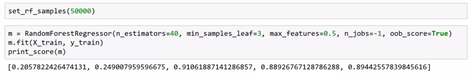
keep your model analysis fast and light at first
In very large dataset using RandomForestRegressor(oob_score=True) will slow you down. When Jeremy is at the beginning of setting up his model he likes to test with 50000 observations (aka set_rf_samples(50000)) because it’ll run fast. With a too large sample set–for example if you pass set_rf_samples(1_000_000_000) to the RandomForestRegressor(oob_score=True)–, it’ll take forever (see Prince Grover’s comment for further explanation). At this this point, you might as well have a proper validation set.
Once you get your preliminary results about your error rate from the RFR, you can start playing with the [different parameters]. Here’s is a pretty clear walkthrough of the parameters of the Random Forest Regressor. You can tweak any of the parameters with the goal of bringing down the error rate.
Q: what does the n_jobs parameter do in RandomForestRegressor (RFR) model?
n_jobs Is number of cores the model will use. n_jobs= -1 means use every single core in the cpu. If you’re running several models, you might want to specify the number of cores a RFR can use.
Light and fast can still give good results. A Favorita competitor in a Kaggle kernel took the average of each item across last 2 weeks as predictions, and then submitted these averages data and scored 30th on the leaderboard. Good enough can get you pretty far.
The question is what can you do to score better than some basic data transformations or out of the box random forest. If you can be a tiny bit better, you can jump up on the Kaggle leaderboard.
Building a robust validation set
If you don’t have good validation set, it’s hard to create a good model. You need to build a validation that you know is reliable in telling you whether your model is performing well or not.
In general, one should not touch/look at test set until right at end of the competition or project . One exception is for calibrating our validation set in a Kaggle competition. For example, Terence Parr made a few subsets to test for accuracy against the leaderboard by submitting. He found a sample set that performed about as well as the test set. With a trustworthy validation set, you can score your models against it quickly, tune all the parameters very quickly without using the test set.
Designing the validation set involves iterating the validation set: looking at the test set and drawing out or plotting out similar features in the test set that can be found in the training set In creating his validation set, Professor Parr looked at date range of the test set and then noticed that the test set was 16 days and started and ended on a payday. In other data sets, you’ll be looking for big spikes when plotting the features of the test sets and different samples of training data that you’re considering for a validation set.
interpreting ML models. how confident are we of a prediction? less confident if we’ve not see many rows like this one. Take stddev of predictinos of trees. if high, means each tree is giving a very diff estimate of this rows prediction. If common row, we’ve have tighter stddev.
Using Kaggle to practice how to code and how to think about problem
Coding for machine learning is hard, not in the traditional software engineering sense. But it is incredibly frustrating. As the the data scientist thinking about what to do isn’t intellectually difficult. instead it’s “how” to execute the idea; how to decide which new information to introduce to the model; there are details that are difficult to get right.
If you’ve made a mistake in executing these detail, you won’t get an exception thrown; your model will silently be slightly less good than it could’ve been. At least with Kaggle, you have a benchmark in the leaderboard by which you can judge your model. In real-life data situations, you simply don’t know if your model can be better.
Kaggle competitions gives you practice on finding all little things that will screw you up.You need a situation where you everything button you press is wrong, and that way, over time, you learn what to watch out for next time. But with every submission, you have a chance to have immediate feedback so you can direct the ways you can improve. For example, you can try to add external data, such as weather data, to your Kaggle models (as long as the data is public and shared with the other competitors) to see if that improves your model. In real life situations, you should always be on the lookout for external data to add (see Kaggle Rossmann Stores competition winner’s strategy of creating more columns of data)
Interpreting Machine Learning Models (aka Models do more than predict)
We’ll come back to the Bluebook for Bulldozers data to see how can use a machine learning model’s results to provide more information than predictions. In addition, to wanting to know a prediction, we want to know how confident we can be about those predictions.
Confidence Intervals based on standard deviation:
If a trained random forest model sees a novel datapoint, the tree/estimator that assesses it will treat it differently than the information it has already seen. It may end up on an outlier branch of the decision tree. If we only use confidence intervals based on averages, the novel data point won’t be judged accurately. Instead we can use, standard deviation of the trees’ prediction to provide confidence levels for the predictions. If standard deviation is high, this means each tree is giving a very different estimates of this rows’ prediction. If the observation is judged to be a very common kind of row, we’ll have tighter/smaller standard deviation score.
Confidence intervals can help you learn about which groups or features the model may not be confident about.
sklearn doesn’t have such a library that outputs the standard deviation of trees’ prediction, but we can make one. We’ll need a good enough RFR model with 50000 observations as a sample set. (for code and procedure: see 58:25 in class video)
Taking the standard deviation of all the trees in the RFR take a long time, but from the fastai library, we can use parallel_trees(), to get the standard deviation across the trees’ prediction.
Taking the standard deviation of the trees’ prediction can help us explore the unknowns about the data set. We’re looker at Bluebook for Bulldozer data, and after plotting the trees’ predictions and confidence intervals with the difference buildozer features, we can do exploratory data analysis on what’s important even when we don’t know what the features is exactly. For instance, the “Enclosure” feature of bulldozers is something that we don’t know what the values means right now, but we after the plots we know that it’s important. The bar charts of the confidence levels gives us an intuition behind how to apply different feature groupings and we can identify which features contributed to low prediction accuracy. Are there some groups that the model isn’t confident about? This confidence value could also be used in as an end product, like in loan application. We could judge yes/no on giving a borrower a loan, and we could also provide a confidence level on whether or not the borrower will pay it back.
Feature importance :
To determine feature importance, you would build a RFR as fast as you can. You’re aiming for an accuracy score better than random, but not much more than that. Then you would plot the feature importance of the different fields in the analysis
Which features matter in random forest ?
- Use
rf_feat_importancefrom the fastai library which plots top features based on their importance
feature_importance = (rf_feat_importance(model, training_dataframe); feature_importance[:10](the code is built on top of sklearn)
The function will picks out the top 10 features in the analysis in order of importance
If you plot all the columns, you’ll find that some columns are important, and some don’t matter at all. ‘Enclosures’ does score as being important, so we’ll have to learn more about enclosures on bulldozers. Understanding which features are important directs us where we to need to gather domain knowledge. This is the part where you sit down with a client and ask about the key features. You would do exploratory data analysis on key variables: run different plots or significance tests. If the feature reveals itself to be important for prediction and client says it’s not, this could indicate a data leakage.
Feature importance analysis might also find co-linearity in variables, so we might see a few features that are appear important but in fact signal the same thing or a similar trend. You have to be careful with your analysis if you see this happening. One experiment is to start throwing data out of the analysis to see if anything changes in your prediction. In our bulldozer experiment, we’ll exclude any feature that scored lower than .005 importance. We can create a new dataframe using only these top features; we’ll divide this slimmed dataset into a test and train sets and pass these to a new RFR instance. Instead of dropping, the accuracy of the RFR actually increased after throwing out less important features.
Generally, throwing out redundant columns shouldn’t make your model worse; if accuracy goes down, those columns weren’t redundant after all. Tossing out redundant columns also lowers the possibility of collinearity (aka two columns that may be related to each other). In a random forest, the tree will mistakenly group different features together because they’re similar.
Understanding the important features of a dataset lets us concentrate on what matters and will make our models run faster. By removing low impact variables, we make our feature importance plots clearer, we can trust these features’ importance more.
Surfacing data leakage can be useful
What is data leakage? – A feature of the data becomes available that was not originally intended when the original data was input or when the dataset released. In other words, there’s information about dataset that you have that the client didn’t have at the time the dataset was created.
This unintended feature can be surfaced during data exploration and interviews with the data stakeholders. For example, Jeremy worked on predicting successful applications for a university grant program, and he found out a single feature–whether the applications were submitted or not, determined whether a grant was was funded. However, he talked and listened to all the people involved in the dataset’s creation. He discovered due to the fact that it was administratively burdensome to log the data around the grant applications, administrators only entered successful grants into database. To make a valid model, this feature needed to be left out of the analysis.
Understanding data leakage is important because either this data leakage feature leads the analyst to make a mistaken conclusion or to build an inaccurate model. Investigating data leakage takes legwork and exploration that may lie beyond the data in front of you. On the other hand, a data leak can used as additional feature to make a better performing model in some situations (i.e. Kaggle competitions).
Jeremy’s Machine Learning trick of the day
Here’s a technique that applies to all machine learning models that nobody seems to have written about. It’s often used with Random Forests, but works with all models.
For example, let’s use our bulldozer examples. We have ‘year_made’ amongst our 25 important variable about bulldozers. How do we figure out how important is ‘year_made’ in our set of 25 features? We organize this data and pass it through a RFR and find out we have an accuracy score of .89.
To explore how ‘year_made’ or some other some variable/feature is affecting our model, we permute the column of interest by shuffling it (the max, min, mean and std deviation remains the same, but we’ve destroyed the feature’s relationship with the other data). We pass this perturbed dataset to same random forest model and do predictions, and we find out the accuracy score is now .80. So we’ve learned that ‘year_made’ is responsible for .09 of the accuracy of the model. We now know it’s feature importance score. We can systematically shuffle each of the 35 categorizes separately to get the feature importance of each category.
While we could also remove year_made (or any column of interest), and pass the amended dataset into it’s own RFR. Then we will have to retrain our random forest over and over because we’ve changed the data it sees. With this targeted shuffle approach, we can just do predictions using same model without retraining it, which is much faster. You can also use this technique to see which pairs of variables are important by destroying each pair of features in turn (but in practice, this paired-shuffle is computationally expensive, and there are better ways of doing it)
Other questions
Q: How does 1 decision tree in default random forest takes sub sample or does it train on complete data?
If bootstrapping = False then it takes all samples without replacement. So it will have all the raws. If bootstrapping = True then it will take len(df) rows but with replacement. So there will be duplicates which make each tree different. Default is True
For homework:
- Go through different styles of plots and find out if there’s anything we can learn about the grocery data,
- Is there anything about this data that we can draw new insights from. Is there any information we may be able to split out into it’s own column ( i.e. is there a different way to split out the dates that might be more meaningful)
- Is there other external data that would give us insight into the current dataset.
- Have a think about what features we can implement and hopefully you’ll come up with a better score by class on Tuesday
.
(Hat tip to Terence Parr, Prince Grover and Tim Lee for contributing their notes and insights! Thank you for sharing!)