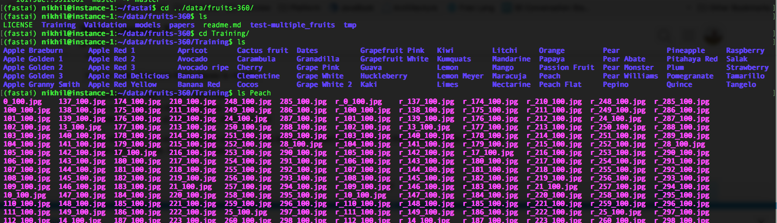
Hi guys, I could not find the file/folder that contains label information for cats/dogs classification in the dataset. How does the model learn without labeling?
Edit: I found that all cat images were put in one folder while dogs in the other one, probably they were labeled in this way, which I am not quite familiar with.
Would you share your code for the kaggle dog breeds competition using fastai libraries? Because I found that code used label data while the code for dogscats did not. Thank you.
For the instructors, I wish there was a half-completed notebook with tasks/notebooks that I could fill out for this lesson. I am not very clear what to do after watching the lesson. Right now I am playing with the notebooks, but without much direction.
Edit: I started watching lesson 3 and I see there’s a task to classify dog breeds using the kaggle dataset, i will do that
This seems like a basic question, so please point me to the right place if I’ve missed it somewhere else
We cover multi-labels in lesson three, but how do you handle multi-classes when one class is unknown? For example, for image classification what would be the set up for “apple”, “banana”, “anything that’s not an apple or a banana?”
I see. From what I’m seeing on Stack Overflow, the solution is to create a “garbage” class that you fill with everything else. Seems like a lot of extra work for something that must be a common problem, but I’ll try it and see.
In lesson 1 @jeremy used the following differential learning rates with the preceding layers trained 10x slower than the following set of layers:
lr=np.array([1e-4,1e-3,1e-2])
In lesson 2 in Understanding Amazon from Space:
lr = 0.2 lrs = np.array([lr/9,lr/3,lr])
While I understand the rationale behind having varying learning rates I can’t seem to understand why lr/9 and lr/3 are used in this case (9 and 3 seem quite arbitrary, why not lr/25 or lr/16 or any other numbers?)
Since we will not want to alter the weights of the earlier layers too much since they capture fundamental low-level patterns / gradients etc. in the images, why are we training it at much higher learning rate in the notebook used in lesson2 vs the dogs-cats problem in lesson1? Only reason I can think of is that the model has been trained on data similar to the data for dogs-and-cats and not on satellite images and therefore we might want to nudge the weights in the earlier layers a little more, but then again how do I know how large a learning rate should be set for the earlier layers?
@henrywjr I think you’re thinking about things the right way–I can’t remember where in lecture Jeremy covers this, but he says pretty much exactly what you describe.
Picking 3 and 3^2 is definitely a bit of a judgement call, but the thinking is just that we want to give the weights more wiggle room. We were using 10 and 10^2 before, and 3 < 10, so Ultimately this is a hyperparameter. You either try a bunch of different approaches and see how they do on your validation set, or you can just follow your heart.
This is regarding Multi-label Classification (lesson2-image_models.ipynb):
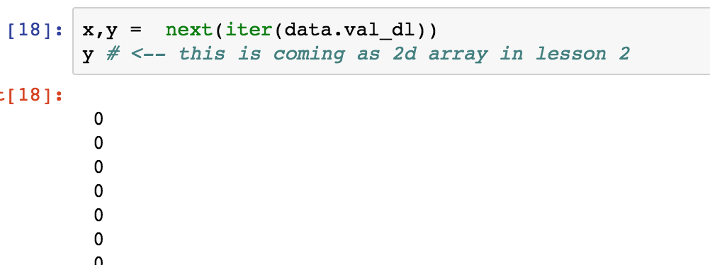
x,y = next(iter(data.val_dl))
Looks like y is a 64 x 17 matrix, it would have made more sense for it to be a vector of length equal to number of classes, so, 1 x 17 or 17 x 1. Why is y a 64 x 17 matrix, what does it represent?
Thanks!
Edit: This was answered in Lesson 3, basically y is the transpose of mini-batch, in this case mini-batch size is 64.
@jeremy chose satellite imgs just to point out that kind of qualitative difference.
When you trained the earliest layers of Resnet over your dogs/cats dataset, you did set TWO orders of magnitude difference with respect to the last two layers (the ones added by us). That was because you did NOT want to spoil those layers’ weights: dogs and cats are very similar to Imagenet’s images over which they were laboriously tuned over.
The same holds, to a lesser extent, for the middle layers (one order of magnitude): the ones that recognize slightly more complex patterns.
Now, you got to unfreeze and train earlier and middle layers over images that are more qualitatively different from imagenet’s images, so you got perturb them a lot more.
Indeed, if lr = 10^-2 is the learning rate of late layers, lr/9 is a lot MORE than lr * 10^-2 ( = 10^-4), and the same stands for 10^-3 vs lr/3 (that is, 10^-2 * (1/3) ).
The gist is that the more you have to cope with images qualitatively different from those used for pretraining, the more you have to be strong on trying higher learning rates.
Hi all. I had a couple of points of uncertainty after Lesson 2 that I would like to clear up before moving on to Lesson 3. (Where they may well be answered.)
I understand that data augmentation takes each training image and applies a random visual transformation to it before using it to train. When augmentation is specified in get_data and precompute is true, does fit() then automagically refrain from applying augmentation and rather precompute activations using the original images? Or is augmentation applied to each training image once to precompute the activations used to train the last layer? The former makes more sense.
The pre-trained resnext in its last layers takes a large number of activations (features) and maps them to a thousand category activations, which are in turn scaled by softmax into a probability distribution across the categories. As I understand it so far.
Our dog breed classification problem starts with resnext, freezes most of it, and classifies images across 120 categories. I see this process described variously as adding a layer, as retraining the last layer, and as retraining the penultimate layer.
What exactly is happening here? Are we training a new layer that takes the thousand ImageNet category raw activations and reduces them to 120 breeds, followed by softmax? Or are we replacing resnext’s one thousand category (outputs) layer with one that maps the same incoming activations down to 120 breed categories, and applies softmax? The latter, I hope, otherwise I am quite confused.
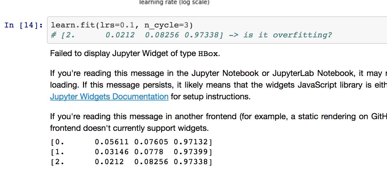
No, I don’t think this is over fitting, which would be defined as a continued lowering of training set loss, which causes an inverse increase in validation set loss. The mental “model” for over fitting is that the model learns the examples in the training set to the determent of generalization. Hope this helps! Adam


 Ultimately this is a hyperparameter. You either try a bunch of different approaches and see how they do on your validation set, or you can just follow your heart.