@jeremy chose satellite imgs just to point out that kind of qualitative difference.
When you trained the earliest layers of Resnet over your dogs/cats dataset, you did set TWO orders of magnitude difference with respect to the last two layers (the ones added by us). That was because you did NOT want to spoil those layers’ weights: dogs and cats are very similar to Imagenet’s images over which they were laboriously tuned over.
The same holds, to a lesser extent, for the middle layers (one order of magnitude): the ones that recognize slightly more complex patterns.
Now, you got to unfreeze and train earlier and middle layers over images that are more qualitatively different from imagenet’s images, so you got perturb them a lot more.
Indeed, if lr = 10^-2 is the learning rate of late layers, lr/9 is a lot MORE than lr * 10^-2 ( = 10^-4), and the same stands for 10^-3 vs lr/3 (that is, 10^-2 * (1/3) ).
The gist is that the more you have to cope with images qualitatively different from those used for pretraining, the more you have to be strong on trying higher learning rates.
Hi all. I had a couple of points of uncertainty after Lesson 2 that I would like to clear up before moving on to Lesson 3. (Where they may well be answered.)
I understand that data augmentation takes each training image and applies a random visual transformation to it before using it to train. When augmentation is specified in get_data and precompute is true, does fit() then automagically refrain from applying augmentation and rather precompute activations using the original images? Or is augmentation applied to each training image once to precompute the activations used to train the last layer? The former makes more sense.
The pre-trained resnext in its last layers takes a large number of activations (features) and maps them to a thousand category activations, which are in turn scaled by softmax into a probability distribution across the categories. As I understand it so far.
Our dog breed classification problem starts with resnext, freezes most of it, and classifies images across 120 categories. I see this process described variously as adding a layer, as retraining the last layer, and as retraining the penultimate layer.
What exactly is happening here? Are we training a new layer that takes the thousand ImageNet category raw activations and reduces them to 120 breeds, followed by softmax? Or are we replacing resnext’s one thousand category (outputs) layer with one that maps the same incoming activations down to 120 breed categories, and applies softmax? The latter, I hope, otherwise I am quite confused.
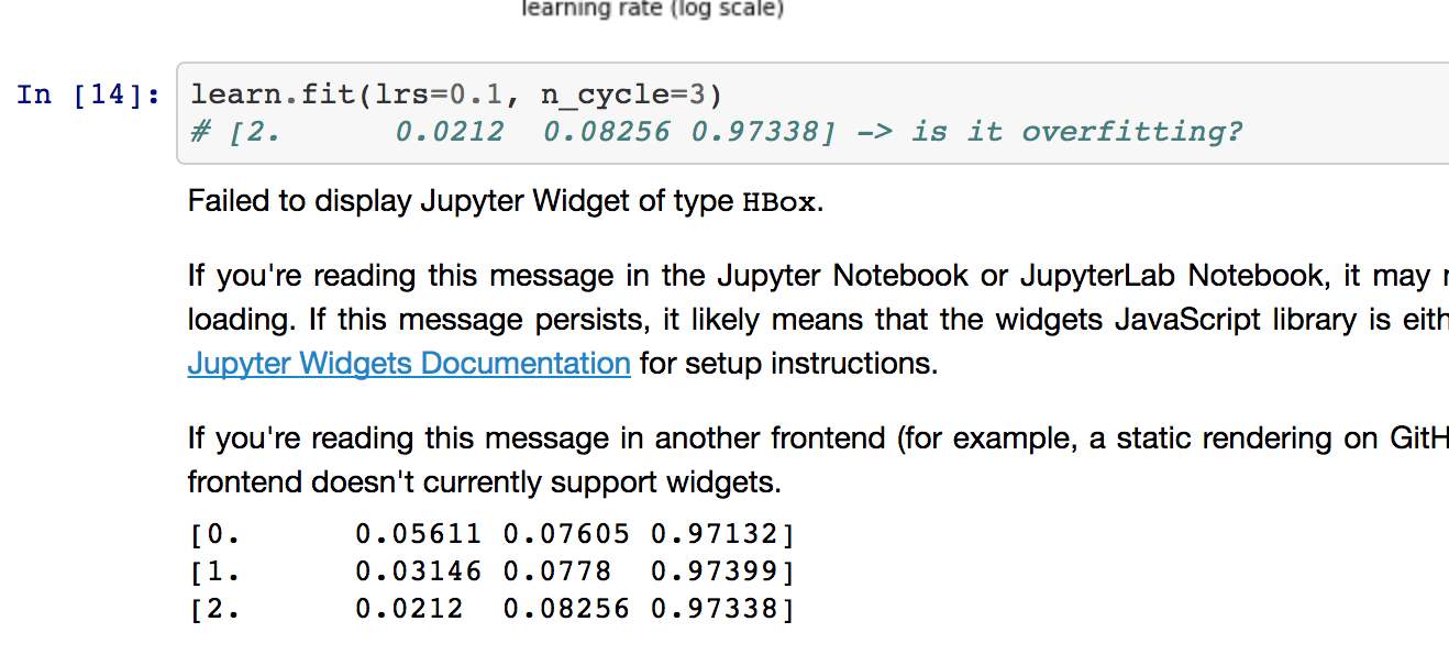
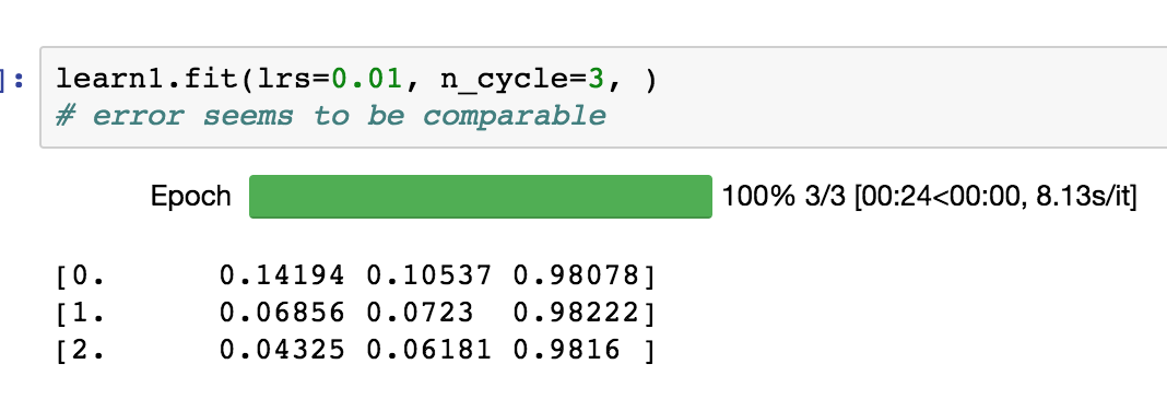
No, I don’t think this is over fitting, which would be defined as a continued lowering of training set loss, which causes an inverse increase in validation set loss. The mental “model” for over fitting is that the model learns the examples in the training set to the determent of generalization. Hope this helps! Adam
Thanks, @wespiser. This is a new perspective. My mental model was if Validation loss was greater than training loss it can be a case of overfitting. I was not sure how much validation loss should be greater to say it is overfitting.
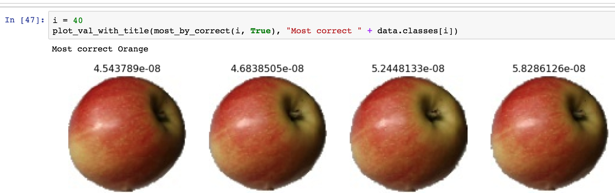
Now I have got my notebook working.. It seems to be correct apart from printing images for the wrong classification.
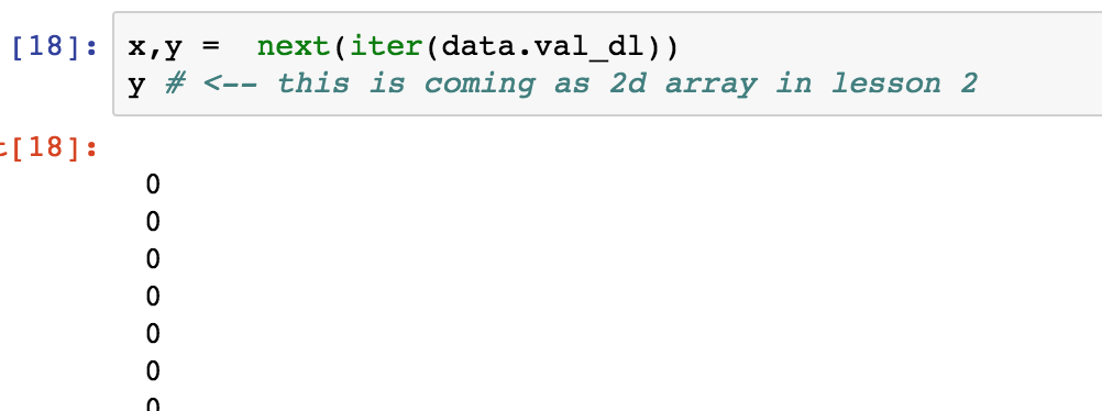
One of my own doubt was why y is 1D array. When we are reading data from csv the give us 2D array. When we read from file system we get a single array.
This small project helped me to learn a lot.
Edit: Another thing to mention is that, using fast I got accuracy of 0.986533717. In comments they have mentioned accuracy from 88% to 98%.
I am listening to the explanation of the learning-rate-finder, and I wonder if there is a good theory on how the magnitude of the gradient changes across its domain?
Given that this learning-rate-finder starts with such a high loss, it seems that we are moving through the domain of the gradient as we vary the learning rate. Therefore it would seem that this program would only have validity if the overall magnitude of the gradient was relatively constant throughout its very large space/domain. Is there any evidence that suggests that the magnitude of the gradient is anywhere close to constant throughout its domain?
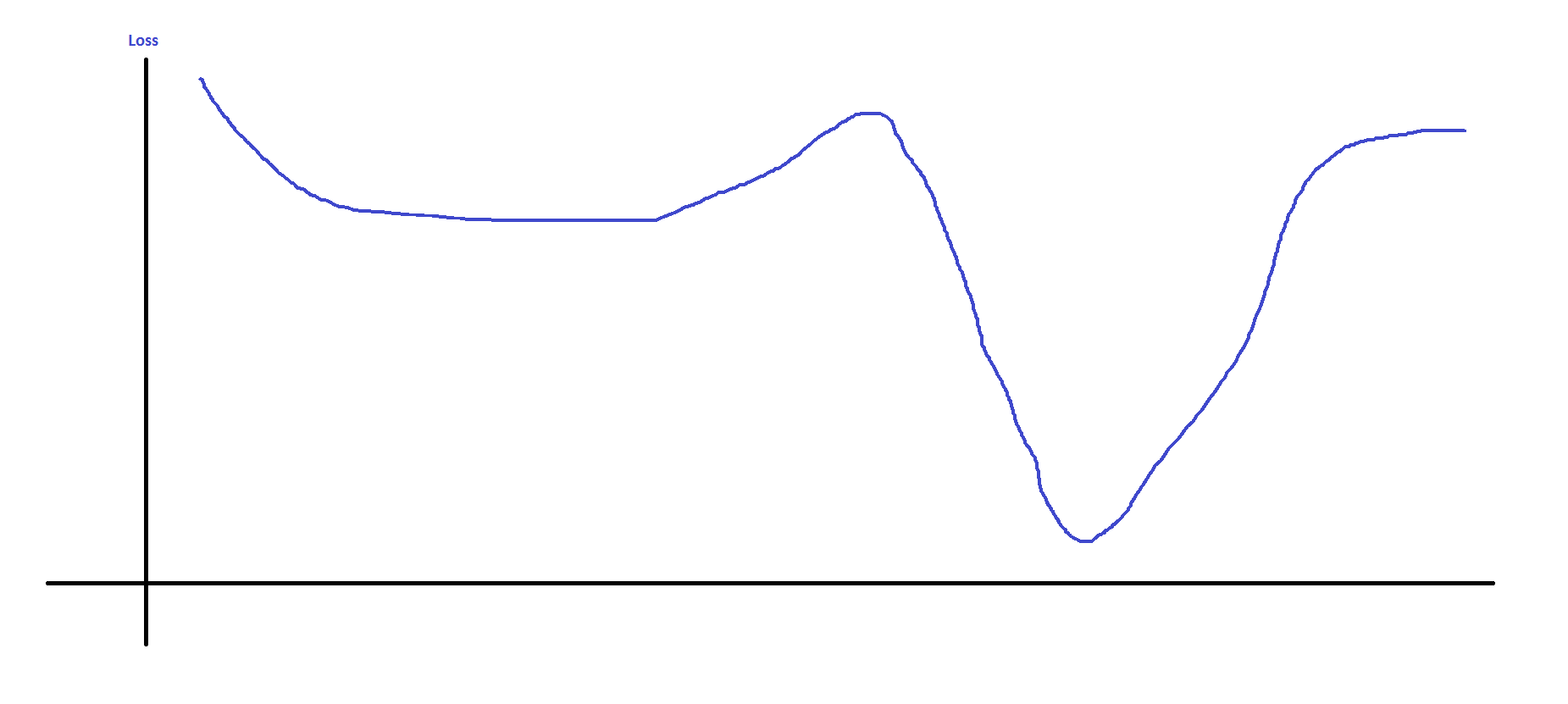
I have drawn a picture to provide an attempt to explain my question with a loss-function that varies only in one dimension. My questions is, do loss functions ever have shapes like this such that the magnitude of the gradient varies across the domain?
We are not moving through the domain of the gradient for the lr_find() method, we are moving loss space.
What the lr_find() method’s domain, or input, is a learning rate, and it’s range, or output is a loss, calculated using the neural network and a few epochs. The idea is that we just want to find a range of useful learning rates to plug into our cyclical learning rate algorithm.
As it was described and to my understanding, the weights of the network are not reset as the learning rate is incrementally increased. Therefore, the network’s weights and biases are different for each chosen learning rate. Since the gradient is a function of the weights and biases (its inputs/domain), changing the weights and biases inherently moves through the space/domain of the gradient, because the weights/biases at the start of each learning rate increment are different. (Unless they are reset each time the learning rate increases)
The important equation is
Weight[t + t] = Weight[t] - learning_rate * gradient(loss)
And section 3.3:
There is a simple way to estimate reasonable minimum
and maximum boundary valueBoth the learning rate, and weights Both the learning rate, and weights Both the learning rate, and weights s with one training run of the
network for a few epochs. It is a “LR range test”; run your
model for several epochs while letting the learning rate in-
crease linearly between low and high LR values. This test
is enormously valuable whenever you are facing a new ar-
chitecture or datase
So, to answer your question, this measure is a heuristic, and doesn’t have any theoretical basis, not yet at least. No one really knows what the shape of of the loss function is. There’s some evidense that most deep neural networks have one global minimum, even though they are incredibly high dimensional space.
I would also look up Stochastic Gradient Descent, its a pretty simple algorithm and we lack a satisfying answer for why it works so well for convolutional neural networks!
has these time estimates [1:48:10<10:49:01, 6490.32s/it], so this part is expected to finish in 10+ hours.
What else is missing? Also, there is hardly any GPU load while running this code, is it possible that the notebook kernel is not using the GPU correctly?
Edit: Solved by restarting the kernel, now it completes within minutes.
I restarted the kernel and it is much faster now. But the cause is still unknown for the problem (ConvLearner running very slowly or not using the GPU properly)
At around the 1 hour 30 min mark of the video, I saw this when the video was talking about making a histogram for the heigh of images and width of images: row_sz, col_sz = list(zip(*size_d.values()))
Can someone explain what is happening here and how 2 different values are able to be assigned?
Also in this line of code in the get_data function: return data if sz>300 else data.resize(340, ‘tmp’), what is the ‘tmp’?
And finally, how exactly does the accuracy(log_preds, y) function work?
When running the Lesson 2 notebook on Crestle, I got the following error: “FileNotFoundError: test-jpg folder doesn’t exist or is empty” after running the following cell: “data = get_data(256)”. I fixed this error by adding the following code into the 4th cell near the top of the script: “!ln -s /datasets/kaggle/planet-understanding-the-amazon-from-space/test-jpg {PATH}”.
Hopefully this is helpful in case if anyone else is having the same issue.