Why do we care about resilency of where we are in the weight space?

I do not know if the reasoning below is correct - I am not trying to answer my own question. Would really love if someone could shed some additional light on this and shoot holes into the parts that are not right or provide me with confirmation. I initially set out to write this having only the question but as I started to type and think on this I came up with this reasoning that gives me comfort I somewhat understand what is going on though at the same time I fully expect I could be completely wrongā€¦

In the notebook, it reads:

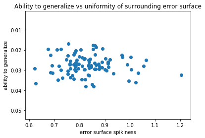
However, we may find ourselves in a part of the weight space that isnā€™t very resilient - that is, small changes to the weights may result in big changes to the loss. We want to encourage our model to find parts of the weight space that are both accurate and stable.

Why would we care about the resilency of where we are in the weight space - isnā€™t low loss the only thing that we care about? Low loss == being close to global minimum.

But in very high dimensional space, local minima are not a concern - any good point with low loss is of comparable quality to global minimum and also it is very unlikely to encounter a local minimum as there (nearly) always exists a way out. Though getting out can be slow (the whole sloshing around the bottom of a ravine idea instead of moving downhill).

Thus I make the assumption that cyclical learning rates are not about getting us out of areas with low loss even if they are not a global minimum (we are not searching for it - we will be happy with any good minimum we find), but for getting us out of areas that would be otherwise hard to navigate? We hope our increased learning rate will get us out of that area (multidimensional saddle point its called?) so that we can try a new area sooner thus shortening the training?

The presuposition is that ā€˜spiky areaā€™, area where small steps in either direction can cause big changes to the loss in either direction, are not very good. A part of the weight space where loss is as low as we can reasonably expect (even though it doesnā€™t have to be a global minimum) will not be like a well, it will be more like a shallow, flat volcano crater?

With adaptive learning rates we were learning how to navigate the ravines better, but with annealing we just say - let me jump around, if this area is good jumping will not hurt too badly, but if it is bad, by increasing the temperature (or in this case just increasing step size) I can hopefully more quickly get to exploring other areas and via getting out of this not so great area quicker I speed up the training?

1 Like

We only care about loss in the validation/test sets. But our training set canā€™t see that data. So we need to know whether slightly different datasets might have very different losses.

Does that make sense?

7 Likes

Yes, it makes a lot of sense :slight_smile: Thank you very much!!!

I keep going back to this answer and I find it extremely eye opening. I can imagine a scenario where a model perfectly (over)fits a given training set based on just one pixel intensity, but this solution would be absolutely useless and had not ability to generalizeā€¦

The notion that we can tell something about our ability to generalize based on the shape of the surrounding error surface on the train set is supercool :slight_smile: and a very useful idea to keep in our mental toolbox. Also, it is interesting to consider this is as a property of various training algorithms, to what extent they not only produce a low train error, but also what measures they take that can help us converge at a nice solution :slight_smile: Seems for the cyclical learning rates it is also a function of how many potential areas we can evaluate in a given timeframe - many more so than we would be able to without the annealing!

Trying not to read into this too much beyond what this idea really entails, but just wanted to stop by and say thank you again for the reply @jeremy! :slight_smile: Appreciate it a lot

2 Likes

Yeah I wonder if you could actually measure how ā€˜spikyā€™ the surface at the solution is, and compare different training methods and architectures to see which finds the smoothest surface.

3 Likes

I think this can be done and would make for a really cool blog post to write :slight_smile:

The easiest and slightly naive way to do it, one could take multiple small steps away from the solution in various directions of the weight space and evaluate the cost. Assuming a 3d weightspace, this would be like projecting a grid onto it from the z-direction and taking a measurement within some distance from the solution at the intersections.

We could sum the squares of the differences in costs or sum absolute values, and compare that against the differences in train cost vs validation cost.

We could then do two things:

  1. See if there are certain training methods that tend end up in less spiky areas.
  2. More interestingly, see if indeed less spiky areas generalize better.

I wonder what would be a good dataset to experiment with this. I would be inclined to use the MNIST, but not sure if it is not too simple? BTW I started playing around with FashionMNIST and I think it is generally perceived to be harder, but I do not know much about it.

Either way, I would be interested in working on this :slight_smile: Sounds like a really cool idea to explore.

1 Like

I think that naive version should be fine. Just pick a few directions at random.

1 Like

@radek My understanding is that. Annealing (w/o the cyclical learning rate concept) is trying to guess when to decay and by how much to decay the learning rate while Cyclical learning rate is more about stability of the minima.

Lets say we are in a ravine (we dont ā€˜knowā€™ how spiky it is). If we keep returning to the same path after the cyclic jumps, it means this is quite stable. If we jump around, that means we are exploring other ravines that may be more stable. My view is that this cyclic jump behavior is orthogonal to the general purpose annealing and both techniques can be used?

1 Like

Note that in the course weā€™re not using cyclical learning rates (CLR), but SGD With Restarts (SGDR). SGDR seems a bit better in my limited testing. Weā€™re using the idea from the CLR paper for how to set learning rates, however.

1 Like

Ah right! I should have said restarts instead of CLR.

I ran an experiment and wrote a blog post looking a bit more closely at this.

There is also an accompanying repository on github with reproducible code (reproducible == open in jupyter notebook and do ā€˜run all cellsā€™ :wink: )

I didnā€™t find what I was looking for which is a bit of a let down but I think there are nice ways to take the experiment further if anyone would be so inclined. This was genuinely fun to work on so I would be tempted also to look at this sometime down the road if time permits.

I also found it quite hard to do some of the things I wanted to do (for instance, looking at gradients) in keras. After just a day of playing with pytorch I can see how it make non-standard things much easier.

3 Likes

Very interesting @radek! What other approaches to measuring ā€œspikinessā€ might be worth trying? Or could you intentionally create some very overfit and some with SGDR etc to have a bigger variance of results to test?

@jeremy - once again you provide me with some very good food for thought :slight_smile: I started typing a reply but I need to think a bit more on the points that you make.

I now see that overfitting might be the way to go. I think I have a design of an experiment in my mind based on this idea that maybe could work quite well.

Doing this in keras is no fun though - I might be wrong, but I think its moving weights to numpy, applying deltas and moving them back to the GPU to reevaluate the model that takes forever. I wonder if the experiment can be run fully on the GPU using something like torch.rand. Possibly also switching the dataset to something like fashion MNIST or CIFAR-10 might also be a good idea - that might be another way to increase the variance.

I posted this on the blog thread but just saw this thread - so the conversation may be better done here. So moving that post here.

I read the post but did not understand it.

Here are questions:

  1. You trained 100 different simple NN on MINST. What is different in each of these NN?
  2. You say ā€˜achieving an average of 94.5% accuracyā€™. Is that average accuracy across these 100? Were all around that number or a large variance?
  3. I understood that now you randomly changed weights and measured resulting loss and compared against previous loss. You took 20 measurements of such change in loss per model. How did you combine these into one number? mean square difference? Absolute sum? % abs change in loss?
  4. In the end I donā€™t understand the graph. The x axis could be the computation in 3 which could be measure of change of loss for small change in weights - so spikiness. Right?
  5. But what is y axis?
1 Like

@radek, very interesting and explicative.

About the experimental design, a couple of ideas crossed my mind (just discard them happily if you find them useless or if have already considered them):

I think your design can be valid, but maybe tricky to implement. First thing I would do: I would compare the NNetworks making sure that they have the same, or very close initial validation error.

Second thought, the more complex a Network is, possibly the more complex its error surface. Maybe one hidden layer is not enough complexity, even it the experiment main insight is simple you need complex surfaces!

Third thought,the scale of the weight distortion is essential. Even then, you dont have that many data points, your chart could well be a part of a bigger chart, possibly even with such small data you get positive or negative correlation number, even if not statistically significative.

So, in few words, very nice post and, if you find the time, I would not throw it to the trashbin yet, not without trying some more little ideas like the ones I gave. Maybe you are already there, you know, I wouldnt be in a hurry to draw conclusions yet. :grinning:

1 Like

By the way, am I the only one who sees an slight negative slope in @radek 's post chart? Maybe my eye is tricking meā€¦ but consider myself good spotting chart patternts. My bet is that you already have negative correlation coeficient. If its the caseā€¦ well you had 50% chances but still I would persevere a bit tuning the experiment and adding more cases!

1 Like

You trained 100 different simple NN on MINST. What is different in each of these NN?
The all share the same architecture, but the weights are initiated randomly - they converge to different solutions after the four epochs. In the weight space, after the training is done, they all end up in different spots.

You say ā€˜achieving an average of 94.5% accuracyā€™. Is that average accuracy across these 100?
Yes, this is correct - this is just an arithmetic mean of the 100 accuracies.

Were all around that number or a large variance?
Yes, the training is very effective - they all were relatively close together though I do not have any numbers that would describe this. The magic - or should I say science :wink: - of batch normalization and adaptive learning rates (both will be covered very soon in this course I think) continues to amaze me.

I understood that now you randomly changed weights and measured resulting loss and compared against previous loss. You took 20 measurements of such change in loss per model. How did you combine these into one number? mean square difference? Absolute sum? % abs change in loss?
I ended up going with absolute sum.

In the end I donā€™t understand the graph. The x axis could be the computation in 3 which could be measure of change of loss for small change in weights - so spikiness. Right?
Yes, you are right - this is the number I obtain in step number 3 by taking 20 measurements for each model and combining them via sum of absolute values.
But what is y axis?
ability_to_generalize_2
For the y axis, the ability to generalize, this is the difference in loss on the train set and the test set. All those numbers were positive - the greater the difference in loss, the lesser the modelā€™s ability to generalize.

I think this is the problem - you need different solutions which very more significantly in how well they generalize.

1 Like

Wouldnā€™t gradient norm give an idea if we land in spiky or flat region ? Given 2 models with similar validation/training losses, would it be a good idea to pick the one with lower gradient norm ?

1 Like

I donā€™t think so - the gradient norm should be about zero when we stop training - but it could change a small distance away.