Hi All,
Yet another update on my satellite project. Yesterday’s lecture about PCA got me thinking about latent space representations for urban characteristics of cities as seen from space.
I tried doing PCA on the later layer’s vector representations of cities, but the results were a little disappointing, so in the end I used U-MAP to do my dimension reduction. It’s much faster than T-SNE and I thought the results were pretty cool.
I also flattened the U-MAP representation to a grid using the lapjv python package which finds the grid representation of distance maps using some fancy algorithm.
Here is the result:
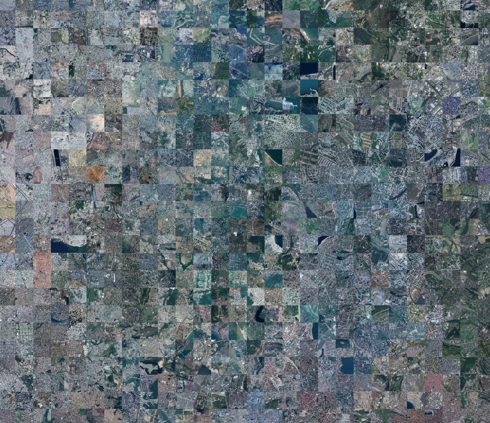
The actual image is 80MB so here are some interesting higher res areas:
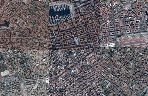
Ochre roofs and twisty roads:
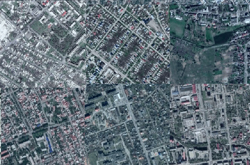
Big backyards:
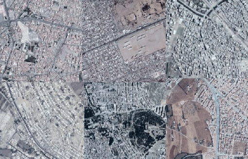
Dense and arid:
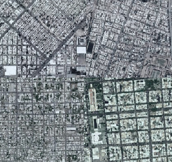
Grids:
You can check the notebook out here