I guess it depends on the goal. If you want to minimise test loss the evidence suggests training the same model multiple times will improve generalisation which will improve test accuracy.
I did try the theory out and it worked for my case. I used Kaggle digits competition specifically for the reason there is a test set which is unknown to the network. I trained the same model 10 times for 40 epochs. I took the model with the lowest validation loss and this yield 99.442% accuracy on the test set. I then used all 400 models (I saved a model for each epoch), run the test set through each and averaged the probabilities. I tried a few different averaging methods (weighted based on validation loss, accuracy, etc). The unweighted average yield 99.528% accuracy. That is an 8.6% improvement. Something I did differently is not throw away the knowledge acquired from each epoch. This idea needs more experimentation. But, anecdotally it suggests every epoch helps.
My conclusion is not withstanding acquiring more data, data augmentation, trialing different network architectures and tuning hyper-parameters (all of which I avoided) predictive performance can benefit from two sources of randomness. The initialisation parameters and the shuffling of samples in each mini-batch. It would be interesting to test each independently.
So if you want to get a boost in predictive performance just train your model multiple times and average the probabilities across all epochs. However, I would only suggest this as the last step after implementing all the other tricks first
I will post a colab notebook. I just need to clean it up.
Hi, I wrote yet another blog about Kaiming weight initialization here. Discussed why it’s mandatory for convergence of your neural model and lots of math from the Kaiming paper. @PierreO and @jamesd blogs were extremely useful. This is my first blog and first paper which I read thoroughly. Any feedback is much appreciated.
So, I tried doing the “A Swift Tour” lesson for Swift beginners, but… it suggested XCode? I couldn’t live with that, so I converted the xcode playgrounds to jupyter notebooks. To make it the most impractical I did the conversion itself in Swift (as I hadn’t written Swift before).
Anyways, you can find the notebooks here: https://github.com/mboyanov/aswifttour . Hope they help someone out
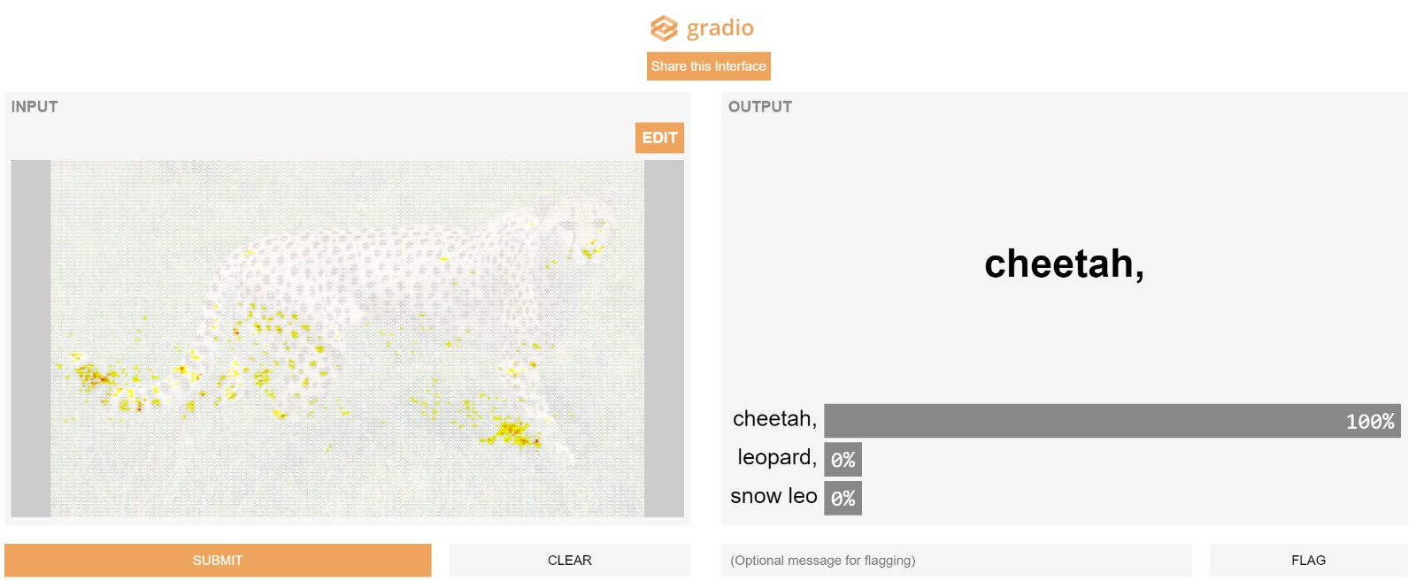
Hey everyone. I wanted a project to strengthen my python. So me and some friends made Gradio.
It’s a python library that let’s ML developers share their model with collaborators and domain experts to be able to use it (and give them feedback!) without writing any code You can create an interface in three lines of code and it will generate a url. (model still running on your hardware!) This is what the url would show:
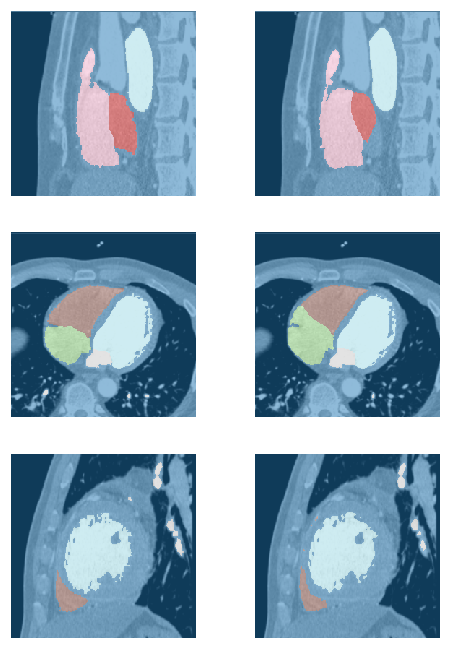
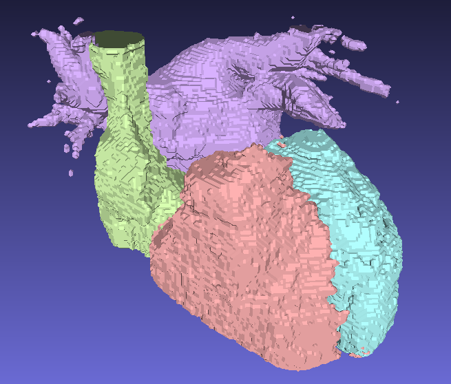
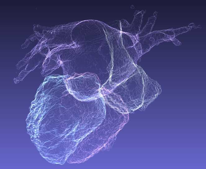
Maybe more of a Part 1 based project, but this is a project I’ve been working on for some of my graduate work. It is a segmentation network that proceeds through a whole CT dicom and highlights the four chambers of the heart.
The base segmentation is just Fastai’s unet implementation. This winds up working pretty well, but you can see sometimes it gets some stuff “wrong”.
The second row is an axial view of a cardiac scan. This is super informative and so it get’s things pretty much right, but things that are difficult to see in one axis are easy to see in another axis. So the first thing you have to do is resize everything to be consistent voxel sizes. Different DICOM scans usually have very different resolutions, especially in the z-axis (head to foot). The next thing I do is just average the outputs of the model evaluating on each plane in each axis.
From the inside of the heart, you can even see which parts are smoother or trabeculated. Pretty fun stuff! I hope you like it. Code is kind of bad and works on some restricted datasets, but I’m hoping to get this working on a public dataset and sharing everything I’ve written for it. If you have any recommendations let me know!
Looks very interesting! You have a labeled medical dataset with these regions highlighted, right? Are you allowed to share some properties about the data and the model, like images resolution, the number of channels, approximate size of the model, etc.? I wonder how long it could take to train this kind of model and which hardware resources one would need.
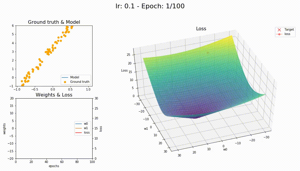
I wrote a post explaining how LAMB works all the way from SGD, including an implementation and some toy dataset explorations.
Edit: Reddit post was deleted, use this instead:
Sure! The dataset is composed of roughly 30 contrast enhanced CT scans where each chamber has been human annotated, stored in this case in h5 files. The scans themselves vary a lot, first the pixel intensities are different for each scanner, and need to be converted to Houndsfield units using metainformation stored in the DICOM. The number of pixel is another problem. They will typically have different numbers of pixels and each will be at a different spacing. Medical imaging is like taking microtome slices down a person from head to toe. When you set the parameters for the scanner, you can set the resolution of each slice (in all three directions) and how many slices to take. More slices usually means more scan time. So people usually space their slices more, so if you were to look at the scan stake into the coronal plane, the scan would be less well resolved, or even squished if you plotted it in matplotlib. This might not normally be a problem if it i were consistent, but it isn’t consistent between scans. And if I ignore this problem, it makes my models take longer to converge, and reduce their quality, and it gets tripped up on new data that is sized differently. So prior to training I go through resizing everything the 3D tensor to be a consistent, say 1x1x1mm voxel sizing.
Another thing is Houndsfield clipping. Hounds field units range from like -1000 to tens of thousands if you have metal around. Eventually this needs to be converted to your standard 0-255 intensities before image normalization, so if you keep that it will put all your useful information in a very narrow tissue range. So best thing to do is just clip it between some set units of interest. That way a pacing lead can’t show up and throw off your scale by a bunch.
This is gray scale, but I just save everything as pngs so it winds up being RGB anyway so I have three channel to work with when I send them back to the network. Otherwise it’s just normal transformations (without horizontal flip) and a normal training schedule, although it’s a lot of data so each epoch takes a while, so I’ve been doing less epochs, max 5 so I can keep prototyping.
Model is just a resnet34 unet! It trains on a regular 2080 GPU over the span of a few hours. So the results you see are just about the fastest, worst results you can get. All the work is in the data in the data preprocessing, as is tradition.
In this case yes! 2D slices being combed from looking through all planes. I’ve tried working with 3D convolutional networks without much success, my batch size is always too small and it doesn’t converge well. This is a while ago though so maybe Jeremey’s new batch norm would fix this problem. Some people have luck with 3D convolutions, but I’ve only heard of that working for bone segmentation, and bone segmentation you don’t even need a network it’s just a thresholding, so that’s probably why it works.
My logic on the 2D approach is that it is kind of how I segment anatomy myself. Most interfaces give you all 3 planes to look at and you can combine your confidence on each to get a good idea on what each pixel should be. (Although it can be really difficult with complex anatomy…) Adding more interslice information would probably work better. One thing I’d like to try in the future is changing the RGB channels to be 3 adjacent slices. To have just a bit more depth context for each voxel.
Hi Poonam, I enjoyed reading your post. It was helpful for me how you dove into the math and step-by-step explained the derivation of the variance/expected value properties behind Kaiming He’s derivation of their weight init formula. I also particularly found helpful your point on ReLUs enabling networks to have sparse representations ー for some reason I’d never explicitly thought of it in this way before.
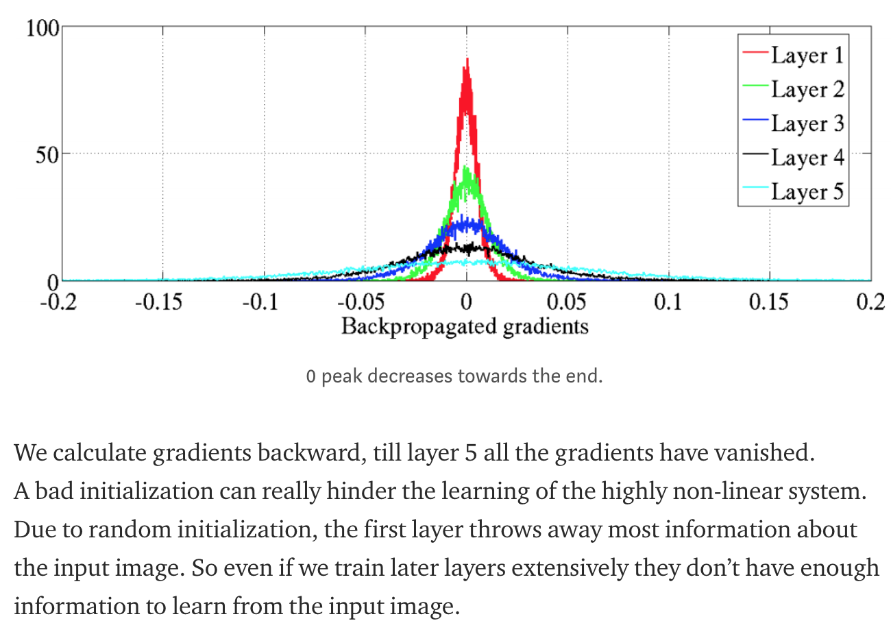
I noticed that when describing Glorot’s vanishing gradients graph, you mentioned that “…till layer 5 all the gradients have vanished…,” while the graph seems to indicate that at layer 5 (final layer) the gradients have a wider distribution, and at layer 1 (first layer in the network) the backpropagated gradients are mostly vanished (they are tightly distributed near zero):
The reason I ask is cause the hardest part of the Glorot paper for me was trying to keep track of whether Glorot and Bengio count layers starting from the network’s beginning (where the input layer is “layer 1”), or do they start counting from the final output layer (in which case the input layer would be “layer 5”)? I think the first approach was what they did.
At any rate, the main feedback I have is something I am also trying to encourage myself to keep doing: please boldly continue to write blog posts and compose tweets
Thanks James for noticing. Yes, input layer is layer 1 and I should have said till layer 1(backward calculation from layer 5 to input layer 1) the gradients have almost vanished. The legend in the graph says it all. I have updated my blog.
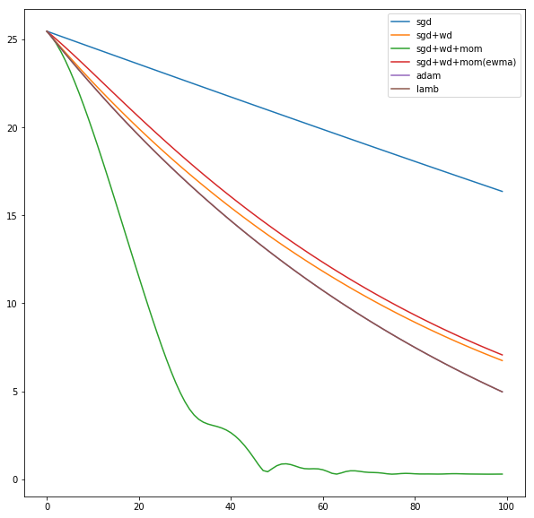
I finally managed to work on something, it is been tough keeping up with this part 2 course. Anyway, I tried to reuse as much of the optimizers notebook to try visualizing them on a sample linear regression problem and comparing the different variations.