Share your work here (Part 2)

I implemented Semantic Image Synthesis with Spatially-Adaptive Normalization (SPADE) by Nvidia which got state of the art results in Image to Image translation. It takes a segmentation mask and produces the colored image for that mask.

It is my first paper that I implemented completely from scratch and got promising results.

Link to repo

9 Likes

I’ve applied ULMFiT to several genomic datasets and shown improved performance over other published results. Currently working on a more long form writeup.

16 Likes

A guy in our study group recently wrote a Medium article on understanding 2d convolution based on CS231n and the paper by He et al 2015.

Felt that it could be of benefit to everyone, so I’m sharing it here with his permission.

An Illustrated Explanation of Performing 2D Convolutions Using Matrix Multiplications

2 Likes

Here is a small Medium Post I wrote on the Instance Normalization:
The Missing Ingredient for Fast Stylization
paper mentioned during Lecture 10.

2 Likes

I was working on kaggle’s jigsaw unintended bias challenge and trained my model using the techniques learned from lessons 9 and 10. Here is my solution kernel. I have tokenized with keras because I am not experienced in nlp with pytorch. I will update my kernel as the time goes on

Today I was thinking about how you might go about discovering a better learning rate schedule.

The first step in my experimentation was exploring what’s going on with the relationship between the learning rate and the loss function over the course of training.

I took what we learned about callbacks this week and used that to run lr_find after each batch and record the loss landscape. Here’s the output training Imagenette on a Resnet18 over 2 epochs (1 frozen, 1 unfrozen) with the default learning rate. The red line is the 1 cycle learning rate on that batch.

static2


And (via learn.recorder) the learning rate schedule, and loss for epoch 1 (frozen) and 2 (unfrozen):

learning-rate
losses-frozen
losses-unfrozen


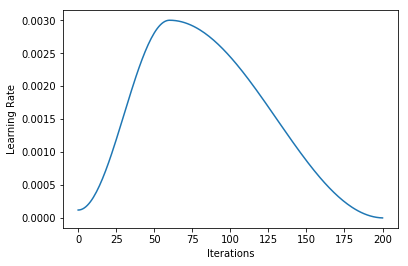
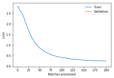
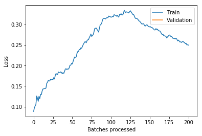
I’m not quite sure what to make of it yet. I think maybe if you could have your learning rate schedule dynamically update to stay just behind where the loss explodes that might be helpful (in the unfrozen epoch I had my LR a bit too high and it clipped that upward slope and made things worse).

Unfortunately it’s pretty slow to run lr_find after each batch. Possible improvements would be running just a “smart” subset to find where the loss explodes and to only run it every n batches.

Edit: one weird thing I found was that pulling learn.opt.lr returns a value that can be higher than the maximum learning rate (1e-3 in this case) – not sure why this would be when learn.recorder.plot_lr doesn’t show the same thing happening.

4 Likes

Great work! Note that freezing doesn’t make sense for imagenette - you shouldn’t use a pretrained imagenet model, since the data is a subset of imagenet, and it doesn’t make much sense to freeze a non-pretrained model.

2 Likes

Whoops! Didn’t even think about that. I’ll have to re-run it again with no pre-training.

Here’s an updated animation showing 10 epochs with no pre-training (one snapshot of lr_find every 10 batches).

It stayed pretty much in the zone! So maybe there’s not actually that much room to improve the LR schedule.

It looks like 1e-3 (which is what lr was set at) would have been good but it overshoots it a bit according to learn.opt.lr – not sure if this is an issue with opt.lr or learn.recorder because they still don’t seem to match up.)

from-scratch2


LR

from-scratch-lr
Loss

from-scratch-losses
Error Rate

from-scratch-error

4 Likes

Great post and notebook on weight init @jamesd :slight_smile: Thanks.

I keep as summary:

  • ReLU as activation function: use kaiming weight initialization
  • symetric non linear activation function like tanh: use xavier weight initialization

Code:

def kaiming(m,h): 
    return torch.randn(m,h)*math.sqrt(2./m)

def xavier(m,h): 
    return torch.Tensor(m, h).uniform_(-1, 1)*math.sqrt(6./(m+h))

Note: in your for loops, you write y = a @ x. You should write y = x @ a (input x that is multiplies by the weight matrix to give the output y) I think.

5 Likes

Wrote a new blog post link. It is based on the paper Weight Standardization.

In short, the authors introduce a new normalization technique for cases where we have 1-2 images/GPU, as BN does not perform well in that cases. They also used Group Norm. Weight Standardization normalizes the weights of the conv layers. They tested it for various computer vision techniques and they were able to achieve better results than before. But they did all their experiments with constant learning rate with annealing after some iters. The main argument is WS smoothenes the loss surface and normalizes the gradient in the backward pass.

So I tested out Weight Standardization for cyclic learning. In the blog post, I present comparisons of with and without weight standardization for a resnet18 model on CIFAR-10 dataset.

But after experimenting for a day, I was not able to get better results using WS. Although, when I use lr_find it kind of shows that I can use a larger learning rate, but when I train the models the results are quite similar. I think the added cost of WS does not justify the performance and for cyclic learning is not a good choice.

Also, if someone can comment on my new blog style. I first introduced the paper, and then showed the graphs for the results. Feedback on this approach would be appreciated.

Someone with experience on Medium, I need some help. When I go to publish my post, they give us an option saying, " Allow curators to recommend my story to interested readers. Recommended stories are part of Medium’s metered paywall.". I just want to keep my blog posts free, so should I use this option.

1 Like

No definitely avoid that.

3 Likes

I modified model_summary a little in 11_train_imagenette notebook to:

def model_summary(model, find_all=False):
    xb,yb = get_batch(data.valid_dl, learn)
    mods = find_modules(model, is_lin_layer) if find_all else model.children()
    f = lambda hook,mod,inp,out: print(f'{mod}\n{out.shape}\n------------------------------------------------------------------------------')
    with Hooks(mods, f) as hooks: learn.model(xb)

then did model_summary(learn.model, find_all=True)
now it prints out the modules and the out shape:


Or model_summary(learn.model):

I thought it was helpful to see in one place how the modules were changing the out shape so I thought I’d share it!

2 Likes

Great minds think alike - that’s what the summary in nb 08 does too! :slight_smile:

FYI you can write this more conveniently as:

f'{mod}\n{out.shape}\n{"-"*40}')
2 Likes

Here is a small Medium post summarizing the BERT training using LAMB paper that was introduced during Lecture 11.
As always, corrections and comments improving the style and content are welcome.

1 Like

Hey, tired of reading how everything went right? Want to see a bunch of AC/DC references shoved into an article?

Then look no further. I did the Kaggle VSB competition about power lines that went horribly wrong for me, and wrote it up here anyway.

1_kPHzKUQMmJ8Y6c8UtdZu5A
That heatmap can’t be right at all!

4 Likes

TfmsManager: visually tune your transforms

I’ve published a tool to quick visualize and tune a complex chain of data transforms (Audio & Image).


15 Likes

How to have a swift kernel in colab:

3 Likes

Ever since getting into deep learning, and making my first PR to pytorch last year, I’ve been interested in digging into what’s behind the scenes of the python wrappers we use, and understanding more about what’s going on at the GPU level.

The result was my talk " CUDA in your Python: Effective Parallel Programming on the GPU", which I had the chance to present at the PyTexas conference this past weekend.

I would love any feedback on the talk, as I’m giving it again at PyCon in ~3 weeks.

15 Likes

Google colab template (link) - exported stuff taken care of so you can pretend you have a local jupyter with all the prev lessons.

3 Likes