Continuing the documentation on the fastai_v1 development here is a brief piece about mixed precision training. A very nice and clear introduction to it is this video from NVIDIA.
What’s half precision?
In neural nets, all the computations are usually done in single precision, which means all the floats in all the arrays that represent inputs, activations, weights… are 32-bit floats (FP32 in the rest of this post). An idea to reduce memory usage (and avoid those annoying cuda errors) has been to try and do the same thing in half-precision, which means using 16-bits floats (or FP16 in the rest of this post). By definition, they take half the space in RAM, and in theory could allow you to double the size of your model and double your batch size.
Another very nice feature is that NVIDIA developed its latest GPUs (the Volta generation) to take fully advantage of half-precision tensors. Basically, if you give half-precision tensors to those, they’ll stack them so that each core can do more operations at the same time, and theoretically gives an 8x speed-up (sadly, just in theory).
So training at half precision is better for your memory usage, way faster if you have a Volta GPU (still a tiny bit faster if you don’t since the computations are easiest). How do we do it? Super easily in pytorch, we just have to put .half() everywhere: on the inputs of our model and all the parameters. Problem is that you usually won’t see the same accuracy in the end (so it happens sometimes) because half-precision is… well… not as precise ;).
Problems with half-precision:
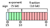
To understand the problems with half precision, let’s look briefly at what an FP16 looks like (more information here).

The sign bit gives us +1 or -1, then we have 5 bits to code an exponent between -14 and 15, while the fraction part has the remaining 10 bits. Compared to FP32, we have a smaller range of possible values (2e-14 to 2e15 roughly, compared to 2e-126 to 2e127 for FP32) but also a smaller offset.
For instance, between 1 and 2, the FP16 format only represents the number 1, 1+2e-10, 1+2*2e-10… which means that 1 + 0.0001 = 1 in half precision. That’s what will cause a certain numbers of problems, specifically three that can occur and mess up your training.
- The weight update is imprecise: inside your optimizer, you basically do w = w - lr * w.grad for each weight of your network. The problem in performing this operation in half precision is that very often, w.grad is several orders of magnitude below w, and the learning rate is also small. The situation where w=1 and lr*w.grad is 0.0001 (or lower) is therefore very common, but the update doesn’t do anything in those cases.
- Your gradients can underflow. In FP16, your gradients can easily be replaced by 0 because they are too low.
- Your activations or loss can overflow. The opposite problem from the gradients: it’s easier to hit nan (or infinity) in FP16 precision, and your training might more easily diverge.
The solution: mixed precision training
To address those three problems, we don’t fully train in FP16 precision. As the name mixed training implies, some of the operations will be done in FP16, others in FP32. This is mainly to take care of the first problem listed aboved. For the next two there are additional tricks.
The main idea is that we want to do the forward pass and the gradient computation in half precision (to go fast) but the update in single precision (to be more precise). It’s okay if w and grad are both half floats, but when we do the operation w = w - lr * grad, we need to compute it in FP32. That way our 1 + 0.0001 is going to be 1.0001.
This is why we keep a copy of the weights in FP32 (called master model). Then, our training loop will look like:
- compute the output with the FP16 model, then the loss
- back-propagate the gradients in half-precision.
- copy the gradients in FP32 precision
- do the update on the master model (in FP32 precision)
- copy the master model in the FP16 model.
Note that we lose precision during step 5, and that the 1.0001 in one of the weights will go back to 1. But if the next update corresponds to add 0.0001 again, since the optimizer step is done on the master model, the 1.0001 will become 1.0002 and if we eventually go like this up to 1.0005, the FP16 model will be able to tell the difference.
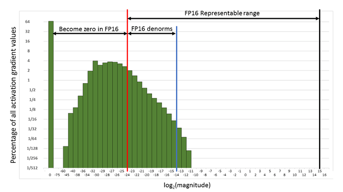
That takes care of problem 1. For the second problem, we use something called gradient scaling: to avoid the gradients getting zeroed by the FP16 precision, we multiply the loss by a scale factor (scale=512 is a good value in our experiments). That way we can push the gradients to the right in the next figure, and have them not become zero.
Of course we don’t want those 512-scaled gradients to be in the weight update, so after converting them into FP32, we can divide them by this scale factor (once they have no risks of becoming 0). This changes the loop to:
- compute the output with the FP16 model, then the loss.
- multiply the loss by scale then back-propagate the gradients in half-precision.
- copy the gradients in FP32 precision then divide them by scale.
- do the update on the master model (in FP32 precision).
- copy the master model in the FP16 model.
For the last problem, the tricks offered by NVIDIA are to leave the batchnorm layers in single precision (they don’t have many weights so it’s not a big memory challenge) and compute the loss in single precision (which means converting the last output of the model in single precision before passing it to the loss).
Implementing all of this in the new callback system of fastai_v1 is surprisingly easy. You can see it in the notebook 004a, and it all fits in one callback where the code is simple to read. In practice, mixed-precision training roughly gives 2x boost of speed. To take full advantage of it check that
- you are on a Volta GPU (which means an AWS p3 instance)
- you aren’t slowed down by the CPU and data aug (it comes faster than you might think)
- the weight matrices have dimensions that are all multiple of 8s (that’s to please the GPUs)
For now, this gets a full training of CIFAR10 to 94% with AdamW and 1cycle in 7min20s in a notebook (baseline is 6min45s, the fastai DawnBench entry). There are a few other tricks to add to get there but compared to 13-14min in single precision, it’s still a huge improvement!
