I’ve tried everything. Different computers, connections, resolutions, etc. No chance.
Maybe a regional issue I’m in Istanbul Turkey. Anyway, I finished re-watching it in four hours that is what matters. ![]()
1 Like
Would love to read this when you publish, I have no idea about devcontainers but I think it would come in handy in other situations I’m dealing with right now ![]()
1 Like
yes, will do!
Just a quick update on using the seeme.ai fastai container. I was able to pull this container and run the diffusion notebook (ssh’d into the container and installed the requirements.txt stuff myself) I also had to map /code in the container to /home/dev/diffusion-nbs coloned repo. I already had the nvidia containers installed as I was running paperspace container .The total container size is about 7GB so it’s not that much smaller than the paperspace fastai container but it’s more recent (about 5 weeks old?)
2 Likes
while playing with the fantastic notebook 9-A by @johnowhitaker, I tried interpolating two latent noise vectors for the prompt “A watercolor painting of an otter”.
I am using linear interpolation to go from random_noise_v0 to random_noise_v1 in 10 steps :
t = torch.linspace(0.0, 1.0, 10)
def linear_interp(t, v0, v1): return (1-t)*v0 + t*v1
I noticed that mixed noise vectors do not produce as good images as the ones generated with non-mixed noise vectors, at the start, and at the end as seen in this gif.
what exactly is the reason for this behavior?
6 Likes
I’ve added the edited video to the top post now.
12 Likes
Wow that’s impressive. May I suggest either you or @mike.moloch consider making a pull request for this since you have the hardware to test the tighter memory constraints? This would doubtlessly be super useful for a lot of people doing the course, and educational as well. Only thing is I know it has a slight performance penalty (about 20%) but I personally think it’s worth being able to run on hardware like this…
3 Likes
It’s certainly the safety filter. For some reason very noisy images tend to trigger false positives, I don’t know what it sees inside all that noise ![]()
1 Like
Starting in diffusers 0.5.1 (released yesterday) there’s a simpler way to disable the safety filter:
pipeline = StableDiffusionPipeline.from_pretrained("CompVis/stable-diffusion-v1-4", safety_checker=None)
This is only meant for experimentation and research, like what we are doing here trying to learn. Please, do not use it in production services, demos or anything facing the public! (You might be breaching the license you accepted).
18 Likes
i came across slerp (spherical linear interpolation) through this amazing repo and got great results with my interpolation experiment. interesting. not exactly sure why this works and linear interpolation doesn’t.
also found this post on reddit that explains the scaling difference b/w lerp (linear interpolation) and slerp which might be the cause.

10 Likes
hey I made a batman comic by curating a bunch of stable diffusion outputs:
12 Likes
In my understanding, the autoencoder and the CLIP model are trained separately. First, you train an autoencoder to learn how to compress images into a latent representation and then train a CLIP model to learn how to associate text with images.
Finally, you freeze both of those models and train the Unet. I’m not sure if I understood your question, though.
4 Likes
I found that UI form that populates in the notebook doesn’t consistently work when I try to submit my token. I can see the requests returning 200 in the browser, but the I would still get a 401 when trying to download the model. To work around this issue, I had to log in via the huggingface-cli with the command below.
huggingface-cli login
Hope this helps.
At about 52 minutes in the video, when Jeremy talks about the gradient of the probability with respect to the pixels, shouldn’t it read something like \nabla_{X=X_3} p instead? Or just \nabla_{X_3} p to keep things simple?
I’m still not through the entire video so apologies if it has been discussed already!
2 Likes
For playing and running the code using colab , check for these two if you get any error.
1- You need to create a token via huggingface and add it to your colab
2- You also need to accept term of service in huggingface
- You need to have huggingface account and log in.
1 Like
Just here to say thank you to @ilovescience and @seem for the 9B lecture that dropped this morning. My first reaction on seeing something with the title “the math of diffusion” was to assume that ‘oh, that’s just something for all the smart people who have PhDs in mathematics on the course, and it’ll probably be completely incomprehensible’, but of course it’s not that at all! I’m not all the way through, but so far I’m just really grateful how you both take things slowly and don’t make any assumptions as to the background of your viewers. So thank you!
17 Likes
I’m having trouble understanding the difference between running intermediate latents through the decoder (in the “Latents and callbacks” section of the Stable Diffusion notebook) and viewing intermediate inference steps (at the end of the “Stable Diffusion Pipeline” section). Shouldn’t these two be the same? What exactly is changing between successive invocations of latents_callback?
Yes, Jeremy has been using \nabla as if it were \Delta. You have the correct notation.
2 Likes
i made a jupyter nb that interpolates between prompt embeddings as well as noise latents. created this animation that shows the evolution of a Ford Model-T to a Modern-day Ferrari ![]()
22 Likes
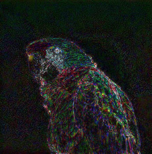
Lesson 9A decoded bird difference
In Lesson 9A Stable Diffusion Deep Dive a parrot image is encoded to latent space and back.
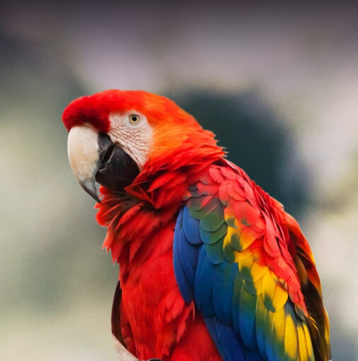
By eye I could not see any difference between the original and decoded images,
but I was curious what a digital difference between the two images would look like.
Its really very subtle, just a little bit of faint colouring. The lack of edges is very interesting:
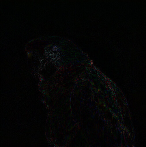
Just for reference, here the differences have been greatly amplifed:
18 Likes