Super cool to see this worked out! Thank you @mkardas!
Also kind of funny that where the Kaiming paper suggests using Var(W_l) = 2/n_l, the neat anwer you got winds up being pretty close to 3/n_l 
Super cool to see this worked out! Thank you @mkardas!
Also kind of funny that where the Kaiming paper suggests using Var(W_l) = 2/n_l, the neat anwer you got winds up being pretty close to 3/n_l
That a[i].unsqueese(-1) was still bothering me as it wasn’t intuitive to me. I found a more intuitive way of expressing it:
# my version
def matmul(a,b):
    ar,ac = a.shape
    br,bc = b.shape
    assert ac==br
    c = torch.zeros(ar, bc)
    for i in range(ar):
        c[i] = (a[None,i].t() * b).sum(dim=0)
    return c
The difference is a[None,i].t(), which is very easy to follow. (1) Take a row vector at index i, (2) turn it into a 2 dim matrix as it originally was, (3) transpose it. Same result as a[i].unsqueeze(-1) but I actually understand how the former does it.
First the full run:
a = tensor([[1., 1., 1.],
            [2., 2., 2.]])
b = a.t()
matmul(a, b)
tensor([[1., 1., 1.],
        [2., 2., 2.]]) a
tensor([[1., 2.],
        [1., 2.],
        [1., 2.]]) b

tensor([[ 3.,  6.],
        [ 6., 12.]])
we get the same results as the original matmult.
Now let’s take the first row of a and do dot product with b step-by-step:
# left matrix
a
a.shape
tensor([[1., 1., 1.],
        [2., 2., 2.]])
torch.Size([2, 3])
# grab a row
a[0]
a[0].shape
tensor([1., 1., 1.])
torch.Size([3])
# turn the row back into a one-row matrix, by restoring the first dimension
a[None, 0]
a[None, 0].shape
tensor([[1., 1., 1.]])
torch.Size([1, 3])
# transpose so that we could do element-wise multiplication
a[None, 0].t()
a[None, 0].t().shape
tensor([[1.],
        [1.],
        [1.]])
torch.Size([3, 1])
# here is the right hand matrix
b
b.shape
tensor([[1., 2.],
        [1., 2.],
        [1., 2.]])
torch.Size([3, 2])
# multiply and sum
a[None, 0].t()*b
(a[None, 0].t()*b).sum(dim=0)
tensor([[1., 2.],
        [1., 2.],
        [1., 2.]])
tensor([3., 6.])
Done.
And also we could reshape the [3] vector into [1,3] matrix with a[0].view(1,-1), so we can also do the prep of a[i] with a[i].view(1,-1).t().
Summary
So the following 4 are the different ways of preparing the row vector from a for an element-wise multiplication with matrix b:
a[i].view(1,-1).t()
a[None,i].t()
a[i].unsqueeze(-1)
a[i,:,None]
I sorted them in the order of ease of understanding for me.
Sweet derivation! I just wanted to make sure I understood your numerical results correctly – you’re saying that shifted ReLU with the initialization scheme you proposed is worse than ReLU + Kaiming, but is not so unreasonable for a large number of states m?
Please don’t hate me for a long post, this is a series of questions that I encountered while studying lesson 8, I have tried my best to read through this discussion and make sure I’m not re-asking something.
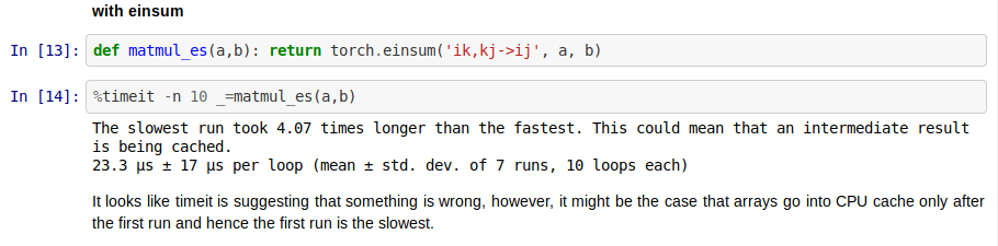
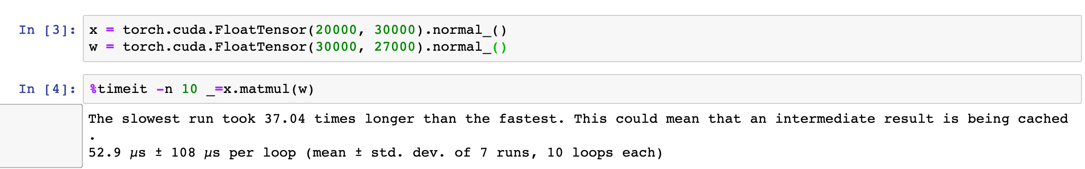
Q1. I tried re-writing the matmul as Jeremy explained and it worked nice, but I always got this extra suggestion with timeit while running on CPU, is there a way to escape it? Does this always happen when we do a model training on CPU?
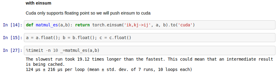
When I do this on the GPU, it still faces the same issue but only for einsum
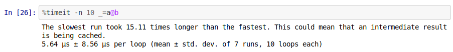
Whereas our manual matmul implementations were fine when pushed to GPU include pytorch’s implementation
ON CPU
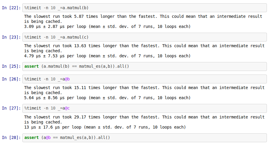
Q2. I took 3 random objects, a,b are both 3X3 and c is 3X1, no matter which implementation I choose for matmul i.e. braodcasting, einsum or pytorch’s, matmul between a and b was always faster and with less deviation that a and c / b and c (ON CPU). Is this just coincidence or perfect matrices operations are faster? and why would that be for CPU and not GPU?
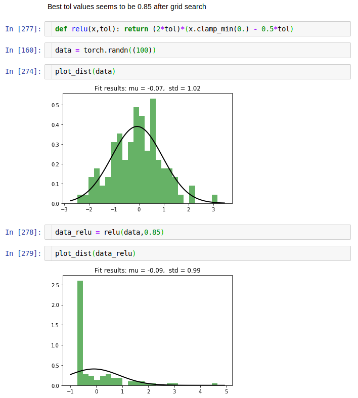
Q3. I was trying to understand the kaiming initialization and modify Relu based on Jeremy’ intuition, I came up with following analysis and deductions
My question is, is it possible to pass tol as a hyper parameter which gets updated? My hunch is Relu can adapt with gradients to better suit (less discard) the data while maintaining the normality. In my small experiments of upto 5 layer network, this is looking better but it is static as we see above. I’m not a stats or math guy but I think an affine transformation will rotate and skew the input space and hence adjusting the height and spread by the same factor maintains the symmetry and we are simply undoing ther effect by subtracting and multiplying.
All the questions and details are from my notebooks available here
Thanks. Yes, that’s one way of looking at this result. But to talk about better/worse I think it would require to compare both in a working network. ReLU with Kaiming helps keep variance from exploding, shifted-ReLU with modified Kaiming additionally helps keep activations mean near 0.
Ah, right on. One thing I never quite understood was – it doesn’t seem that shifted ReLU interacts poorly with the backprop version of Kaiming init… at least I couldn’t figure out how the argument there was different between ReLU and shifted ReLU, since shifted ReLU has the same derivative.
It does seem like I must be missing something, but I do wonder how the numerical results look if we use backprop Kaiming init instead.
Actually, it sort of looks like we specify mode='fan_out' in 02_fully_connected.ipynb, when initializing w1 in the example where we play around with the shifted ReLU (overriding the default of ‘fan_in’). I can’t imagine that’s not intentional… @jeremy do you you know something about this!
Edit: Jeremy talked to me offline and disclaims any knowledge about this – the mode='fan_out' has to do with the fact that the pytorch convention for the weight matrices is the opposite (transpose) of the fastai convention.
Actually, you have very small tensors to reliably compare performance…
Consider sizes of tensors you are measuring performance on. Operations will be parallelized differently depending on your tensor shape for example 10k,1k or 25k,25k for example.
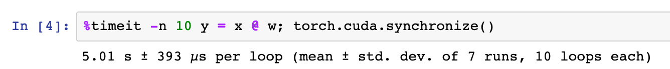
Also measuring timings for GPU is tricky. timeit basically do not give meaningful results for gpu.
Consider:
There is no way it takes 50 microseconds
Consider this:
or
Does anyone know if correlated features (inputs) would make the problem of exploding gradients worse? If not, are you aware of any other issues it might cause, or in general deep NN don’t care about input correlation?
I did some Google search and didn’t get any clear answer one way or another.
Very nice indeed! I did the same thing as you except I’m not statistician enough to have the “common sin of a statistician” 
For those of you that have some linear algebra background (or have taken the computational linear algebra class here) – I asked a (former) mathematician friend about the distribution of the ‘largest’ (in magnitude) eigenvalue for n \times n matrix whose elements are selected uniformly (and independently) from [-1, 1].
He claimed (or his best guess) was that this eigenvalue was O(\sqrt{n}) – which, of course it has to be! Because in all of the initialization schemes we’ve looked at, all of them have a 1/\sqrt{n} in there, and that makes sense because that then cancels out the \sqrt{n} in the largest eigenvalue, which causes your weight matrix to neither scale your layer up nor down by too much.
@sergeman Is there a way you could protect this material from being seen by folks who are not currently in the Part 2 v3 class?
I see this being mentioned in fixup paper. Haven’t read it much though
Before I start with Lecture 2 (9 mod 7) homework, here are a few moments where I had to cheat while doing the homework (replicating notebooks):
require_grad = True to allow gradient calculationHope these gotchas are useful!
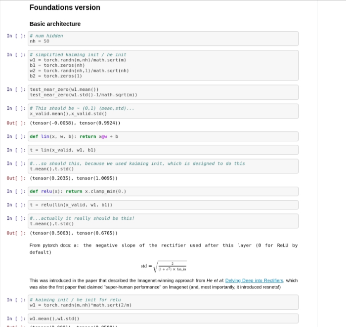
For the kaiming initialization we only multiply math.sqrt(2/channels) with first weights and not second weights. Why is that?
They’re not changing this one - they’re only changing the sqrt(5) init.
Where are you seeing that exactly?
Sorry for getting it wrong, I’ve corrected the OP.
I mean we have initiated w1, w2, b1, b2 but later initialized w1 only as kaiming init / he init for relu
w1 = torch.randn(m,nh)*math.sqrt(2/m)
but not w2 as w1 initialization above.
I’ve removed mention of fast.ai from the Readme.md . The course notebooks are in a public repo protected by obscurity, so they have equal level of protection. I think this should be sufficient.