Lesson 8 (2019) discussion & wiki

[fabris (Fabrizio)]

Hi, better look at A Gentle Introduction to Mini-Batch Gradient Descent so to have a clearer picture.

[hiromi (Hiromi Suenaga)]

@stas

After some thinking I realized that since this function does partial derivatives, then the sum disappears, since the derivative for all entries but the specific input it’s derived for will be 0.

This is a hard concept to really “get it”. I think this is what’s explained in 4.4 of https://arxiv.org/pdf/1802.01528.pdf and after reviewing partial derivative and reading that section many times, it still doesn’t sink in fully.

[wyquek (Qbiwan)]

Not a mathy person to begin with,I read it many times too - bitter but nourishing

[fabris (Fabrizio)]

Sorry, I’d like to help you but I’m a bit confused. Which concept is supposed to be hard to get ?

[jeremy (Jeremy Howard)]

@mediocrates

So it probably depends on how your input data is distributed, but if e.g. the E[y+l]>0.25E[y_l^+] > 0.25, then the variances of your later layers are probably going to be less than that of your earlier layers compared to if you had used plain ReLU

That lines up with what we’re seeing. So how would we adjust the init to account for this?

[mcclomitz (Kieran)]

Im confused about the forward_backward section of lesson 8.

So on the backward pass we run mse_grad() then lin_grad()

Inside lin_grad where does out.g come from? We define out in a number of sections, but what is out.g, where do we get this from?

[hiromi (Hiromi Suenaga)]

I can take derivative of:

\frac{(x-t)^2}{n}

But for something like:

\frac{\sum_{i=0}^{n}(x_{i}-t_{i})^{2}}{n}

The sum disappearing part is not very intuitive to me even though I kind of understand:

@stas

the derivative for all entries but the specific input it’s derived for will be 0

I think it all goes back to this:

A little bit of a hump because I’ve only studied calculus and not matrix calculus.

[hiromi (Hiromi Suenaga)]

The mse_grad function looks like this:

def mse_grad(inp, targ): 
    inp.g = 2. * (inp.squeeze() - targ).unsqueeze(-1) / inp.shape[0]

And you notice that it’s setting inp.g.

In these lines of code, we sent a variable out to mse_grad (which gets assigned to inp inside of the function).

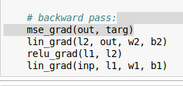
    # backward pass: 
    mse_grad(out, targ)
    lin_grad(l2, out, w2, b2)

So out.g gets initialized inside of mse_grad.

[mcclomitz (Kieran)]

Oh I see – I looked at that for a long time and didn’t see that.

Thanks for your help

[fabris (Fabrizio)]

Actually, matrix calculus sounds weird too. It is proper called it multivariable calculus. About your doubt is about algebraic manipulation and some derivative rule application. Everything starts with

f(x)=\frac{1}{n}\Sigma_{i=1}^n(x_i-t_i)^2

\frac{\delta}{\delta x}f(x)=\frac{1}{n}\Sigma_{i=1}^n \frac{\delta}{\delta x}(x_i-t_i)^2

applying power and chain rule

\frac{\delta}{\delta x}f(x)=\frac{1}{n}\Sigma_{i=1}^n 2\cdot (x_i-t_i)\frac{\delta}{\delta x_j}(x_i-t_i)

the last term on the right goes to 1 when i=j and 0 everywhere else. So we got

\frac{2}{n}\Sigma_{i=1}^n (x_i-t_i)

hope it helps.

[stas (Stas Bekman)]

@hiromi

the derivative for all entries but the specific input it’s derived for will be 0

I think it all goes back to this:

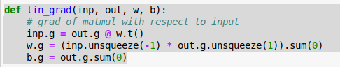
Correct. Because literally what happens with the sum’s partial derivatives is (disregarding the details of the real function):

y      = w0*x0 + w1*x1 + w2*x2 + ...
dy/dx0 = w0    +  0    +  0    + ...
dy/dx1 =  0    + w1    +  0    + ...
dy/dx2 =  0    +  0    + w2    + ...

where wi is just some coefficient (not a weight that we normally are talking about), that is specific to the formula.

And 0’s come because when i!=j those entries are but constants, whose derivative is 0. They are constants because when we take a derivative of y wrt x[i], we “freeze” the rest of variables, inserting constants where all the x[j] (j!=i) variables are, ending up with just y = wi*xi + c. And it’s easy to take that derivative: dy/dxi = wi. That’s how the rows above were built.

So the sum is still there but now it’s summing up all 0’s and one non-0 entry, and that’s why it disappears.

So dy/dx = [w0, w1, w2, ...]

and in the case of mse_grad (x = inp, wi = w[i]):

w[i] = 2. * (x[i] - targ) / batch_size

so once we switch to the vector of derivatives grad we get:

grad = 2./bs * (inp-targ)

Notes:

• this wasn’t an exact math, but was a sort of simplified visual to help understand why the sum disappears, to which I sort of bolted the mse_grad function and it sort of works because mse happens to be a simple sum(c*x^2) function, but in practice you don’t want sort of, therefore once you grok the simplified version, please see @fabris’s answer above for the full rigorous math.

• this demonstration is only true in this particular case where the inputs don’t interact, because if you were to have a different function of a form say y = w1*x1*x2 + w2*x2*x3 then it won’t be all but one non-0 value upon a derivative wrt one input.

• since mse is the first function in the backprop chain it doesn’t multiply its calculated gradient by an upstream gradient. Or you can think of the upstream gradient as 1. These notes can be quite helpful: CS231n Convolutional Neural Networks for Visual Recognition

[PierreO (Pierre Ouannes)]

That lines up with what we’re seeing. So how would we adjust the init to account for this?

I’m note sure there’s an any simple fix here, if \mathbb{E}[x_l^2] is more complicated as described above there’s no longer Var[y_L] = \text{ a nice product}. Or at least I can’t work out one. In this absence of nice math answers (again, maybe it’s just my limitations) maybe the best is to algorithmically search for the best shifted ReLU? I’ll try it if I have time today

[jeremy (Jeremy Howard)]

@PierreO

Or at least I can’t work out one. In this absence of nice math answers (again, maybe it’s just my limitations) maybe the best is to algorithmically search for the best shifted ReLU?

That’s probably best - you can use optim.lbfgs or similar. Or replicate the 90+ pages of math derivation in the SeLU paper…

[stas (Stas Bekman)]

@fabris

the last term on the right goes to 1 when i=j and 0 everywhere else. So we got

\frac{2}{n}\Sigma_{i=1}^n (x_i-t_i)
hope it helps.

Except, there should be no Sigma in the last step the 0’s ate it

\frac{2}{n} (x_i-t_i)

[hiromi (Hiromi Suenaga)]

Thank you @fabris and @stas! I feel like the fog in my brain is starting to lift with the visual of a matrix where everything else but the diagonal elements are zero and i=j

[tamhash]

Hi Everyone!!

I think I got PReLU activation from Kaiming He paper…

class PreRelu(Module):
    def __init__(self,a):self.a = a
    
    def forward(self,inp) : 
         return inp.clamp_min(0.) + inp.clamp_max(0.)@self.a
    
    def bwd(self,out,inp) : 
        inp.g = (inp > 0).float()*out.g +  out.g @self.a.t() * (inp<0).float()
        self.a.g = ((inp<=0).float()*inp).t()@out.g

and ‘a’ needs to be initialized as

a1 = torch.randn(nh,nh)
a1.requires_grad_(False)

I could pass test_near with pytorch’s gradient computations.

Can someone review it and confirm if it makes sense?

[wgpubs (WG)]

This may be a dumb question, but why do we calculate the gradients for x_train in 02_fully_connected notebook since the inputs to our model are never updated?

See:

xt2 = x_train.clone().requires_grad_(True)
w12 = w1.clone().requires_grad_(True)
w22 = w2.clone().requires_grad_(True)
b12 = b1.clone().requires_grad_(True)
b22 = b2.clone().requires_grad_(True)

Wouldn’t it be more proper, in a real world scenario, to set xt2 as such:

xt2 = x_train.clone().requires_grad_(False)

[mediocrates (Justin Shih)]

If, hypothetically, you could pick c = -2E[y_l^+], then (maybe?) things could work out? Does this even make any sense, though? It definitely seems a little strange to have the model depend on the input data, even if only as a shift to each of the different ReLUs. And the y_l also depend on the W_l, so there might be some recursion to work out. Doesn’t seem particularly promising… at least I’m not sure where I would go next with this.

[sgugger]

That was to check all the gradients are correct. Note that we don’t update anything in that notebook, so it’s just for the purpose of verifying the backward computation were all correct.

[mkardas (Marcin Kardas)]

The Kaiming analysis, using notation from your blog post, states that if we use Kaiming initialization and a standard ReLU, then \mathbb{E}(y_l)=0 and \mathop{Var}(y_l)=2. For convenience, let’s init weights of the first layer with \sqrt{1/m} instread of \sqrt{2/m}, so we get \mathop{Var}(y_l)=1 for all layers. Now, instead of ReLU we use ReLU shifted by c and c is chosen so that x_l is centred around 0. Let’s assume that we were able to fix the weights of layers up to l such that \mathop{Var}(y_{l-1})=1 and \mathbb{E}(y_{l-1})=0. Using a @mediocrates formula,

\mathop{Var}(y_l) = n_l\mathop{Var}(W_l)\left(\frac12 \mathop{Var}(y_{l-1}) + 2 c\, \mathbb{E}(y_{l-1}^{+})+c^2\right).

If we assume that y_{l-1} is normal (the most common sin of a statistician? ), then \mathbb{E}(y_{l-1}^{+})=\frac{1}{\sqrt{2\pi}} and

\mathop{Var}(y_l) = n_l\mathop{Var}(W_l)\left(\frac12\cdot 1 + \frac{2 c}{\sqrt{2\pi}}+c^2\right).

To get \mathop{Var}(y_l) = 1 we need

\mathop{Var}(W_l) = \left(\frac12\cdot 1 + \frac{2 c}{\sqrt{2\pi}}+c^2\right)^{-1}\frac{1}{n_l}.

Again, if we assume that y_l is normal, then we should set c=-\frac{1}{\sqrt{2\pi}} so that \mathbb{E}(\text{shifted-ReLU}(y_l)) = 0. Therefore, we should init W_l (except the first layer) with

\mathop{Var}(W_l) = \left(\frac12 - \frac{2/\sqrt{2\pi}}{\sqrt{2\pi}}+\frac{1}{2\pi}\right)^{-1}\frac{1}{n_l} = \frac{1}{n_l (\frac{1}{2}-\frac{1}{2\pi})}.

How incorrect is the normal assumtion?
I’ve tested it with 21 linear layers with shifted-ReLU, with 784 input states and m=50 or m=500 states in the remaining layers. Edit: plots labelled Var actually show std.

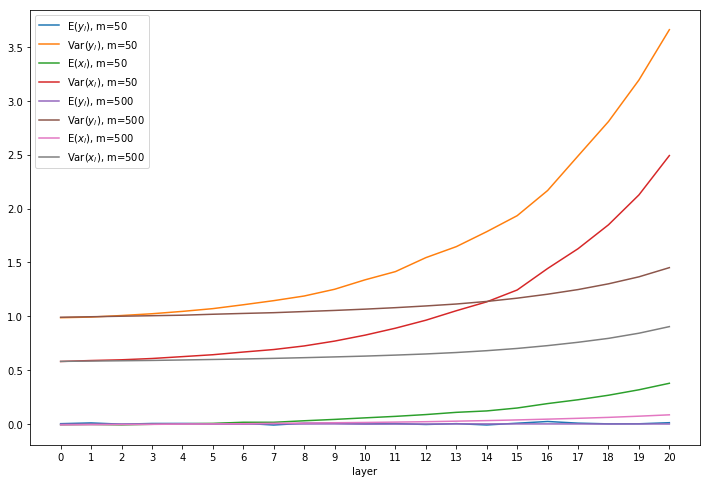
With larger values of m the central limit theorem starts to work and the distribution is more normal. For comparison, below is ReLU with Kaiming: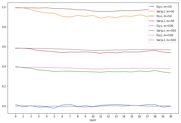

Looks much better, even for m=50.