There’s no relu after the 2nd layer, so no correction needed. Thanks for the good question!
My intuitive response would be the opposite. The NN would figure out the closeness of the relationships between the different co-related input variables and arrive at a faster solution (implying that gradients are not exploding). I currently do not have the data however to prove this intuition.
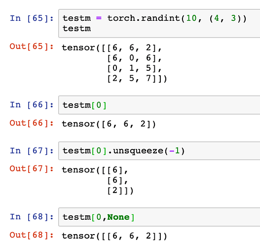
I found this a bit confusing at first too. I think either I’ve misinterpreted the video or Jeremy makes a bit of a typo (speako?) in the instruction. When describing replacing the second loop with broadcasting, he says
c[i] = (a[i ].unsqueeze(-1) * b).sum(dim=0)
could be rewritten as
c[i] = (a[i,None ] * b).sum(dim=0)
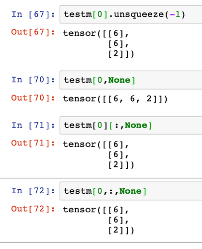
I tested that, and it doesn’t seem to produce the same output:
Perhaps he meant to say it could be rewritten as
c[i] = (a[i][:,None] * b).sum(dim=0)
Which does produce the same output as the .unsqueeze(-1) version. And as you point out that can be further simplified to
c[i] = (a[i,:,None] * b).sum(dim=0)
Perhaps this ought to be an errata? 
(If it was indeed a buglet, it’s good to know that even professional vector reshapers get a bit confused about this from time to time  )
)
It’s in Errata - please see the first post, @ThomM.

I recall Jermey saying something in one of the videos (I believe the ML course) that correlations shouldn’t matter. However, when I did some Google search, a few people were saying it is better to only put in independent features, so that is why I was wondering if they somehow cause issues with training.
Since there is no ReLU after layer 2 shouldn’t we use Xavier initialization instead of Kaiming for w2? If I understand correctly Xavier’s initialization paper analysis was done by assuming there is no activation at all, so it makes sense to initialize w2 by dividing by math.sqrt(fan_in), or am I missing something?
Thanks @maxim.pechyonkin for your response and the links.
I was moving onto some other topics when I came back to this by way of reading the docs for Learner, then the training overview, then learning about callback implementations like PeakMemMetric, and eventually arriving at this Pytorch forum topic about some gotchas with Pytorch/GPUs, unveiled by monitoring during training.
Though I’m nowhere near rigorous understanding, it’s very interesting to see how the pieces come together.
Where does the terminology fan_in come from? I think I understand it is the number of input nodes, but where did that terminology start being used? As far as I can tell, it never is actually talked about in the “Delving Deep Into Rectifiers” paper.
I have a question regarding PyTorch’s .backward() function. Does it calculate local gradients with respect to output of each parameter’s layer’s output or the global gradient with respect to the loss of the model?
In notebook 02_fully_connected, Jeremy calculates local gradients by hand for each layer. Than means w1.g, b1.g, w2.g, b2.g all store gradients with respect to the layer’s output, and not the loss of the model:
def mse_grad(inp, targ):
    # grad of loss with respect to output of previous layer
    inp.g = 2. * (inp.squeeze() - targ).unsqueeze(-1) / inp.shape[0]

def relu_grad(inp, out):
    # grad of relu with respect to input activations
    inp.g = (inp>0).float() * out.g

def lin_grad(inp, out, w, b):
    # grad of matmul with respect to input
    inp.g = out.g @ w.t()
    w.g = (inp.unsqueeze(-1) * out.g.unsqueeze(1)).sum(0)
    b.g = out.g.sum(0)

def forward_and_backward(inp, targ):
    # forward pass:
    l1 = inp @ w1 + b1
    l2 = relu(l1)
    out = l2 @ w2 + b2
    # we don't actually need the loss in backward!
    loss = mse(out, targ)

    # backward pass:
    mse_grad(out, targ) # out.g
    lin_grad(l2, out, w2, b2) # l2.g w2.g b2.g
    relu_grad(l1, l2) # l1.g
    lin_grad(inp, l1, w1, b1) # inp.g w1.g b1.g
Then, he uses PyTorch builtin autograd to calculate gradients, by using:
xt2 = x_train.clone().requires_grad_(True)
w12 = w1.clone().requires_grad_(True)
w22 = w2.clone().requires_grad_(True)
b12 = b1.clone().requires_grad_(True)
b22 = b2.clone().requires_grad_(True)

def forward(inp, targ):
    # forward pass:
    l1 = inp @ w12 + b12
    l2 = relu(l1)
    out = l2 @ w22 + b22
    # we don't actually need the loss in backward!
    return mse(out, targ)

loss = forward(xt2, y_train)

loss.backward()

test_near(w22.grad, w2g)
test_near(b22.grad, b2g)
test_near(w12.grad, w1g)
test_near(b12.grad, b1g)
test_near(xt2.grad, ig )
And all the gradients calculated by hand match those calculated automatically.
I thought that loss.backward() calculates all the gradients with respect to the loss, but it looks like it will calculate local gradients, meaning not w.r.t. to the loss but w.r.t. to the output of the layer where each parameter is used (because this is what is calculated by hand). Am I mistaken?
If I am correct then, for parameter update step, we need to multiply all local gradients by hand, implementing the chain rule? But I haven’t seen that done in examples before. So are the gradients local or global in this example?
Edit: I see now that the chain rule is implemented in the examples done by hand. The local gradient is multiplied by the global gradient out.g, which is the gradient of loss w.r.t. the output of the given layer. I guess my question can be disregarded. Should I delete it?
- the local gradient is always wrt each input of that layer, and then multiplied by the upstream gradient (chain rule)
- mse_grad was an exception of not having upstream, so it gets multiplied by 1.
CS231n Convolutional Neural Networks for Visual Recognition has good visuals.
The local gradient is multiplied by the global gradient
out.g
not sure what you mean by ‘global’, but basically whatever is coming from upstream in backprop (out.g in our examples). see the link above.
If the computation graph were to branch out into more than one output []-< then you’d have to aggregate those upstream gradients in out.g before multiplying by it. I meant something like:
    []
[]=<
    []
as compared to the typical layer sequence that goes in in forward, rather than out:
[] \
    []
[] /
the drawings didn’t come out great by I hope it make sense.
By global I meant with respect to the loss. After I asked the question I realized I wasn’t paying attention to the fact that all local gradients are multiplied by the ‘out.g’ to get the global gradient with respect to the loss.
Thank you, Jeremy.
You are correct.
I don’t know when it first appeared. Maybe you can do some etymology research!..
I think that working through this thought process will be interesting to others - so I’d say no.
Well, I have started down the rabbit hole and unfortunately, I have just replaced one question with another. It appears that the fan_in & fan_out concept is used in hardware when talking about transistors. So it was adopted from there I am quite confident. Unfortunately, that doesn’t really answer the question of why they used the term fan.
My current thought is that maybe it has to do with the number of hardware inputs getting narrowed down to a single chip and that sort of looking like a fan, but that is just a complete guess. I haven’t seen anything that connects those.
Here is my guess though. Maybe somebody else can find something that connects the term fan better.

My current thought is that maybe it has to do with the number of hardware inputs getting narrowed down to a single chip and that sort of looking like a fan, but that is just a complete guess.
From doing some googling it looks like in general in DL it’s the same:
- Fan-in: is a term that defines the maximum number of inputs that a system can accept.
- Fan-out: is a term that defines the maximum number of inputs that the output of a system can feed to other systems.
Here is my summary of these concepts from: http://deeplearning.net/tutorial/lenet.html
For MLPs, fan-in is the number of units in the layer below.
For CNNs however, we have to take into account the number of input feature maps and the size of the receptive fields:
        # there are "num input feature maps * filter height * filter width"
        # inputs to each hidden unit
        fan_in = numpy.prod(filter_shape[1:])

        # each unit in the lower layer receives a gradient from:
        # "num output feature maps * filter height * filter width" /
        #   pooling size
        fan_out = (filter_shape[0] * numpy.prod(filter_shape[2:]) //
                   numpy.prod(poolsize))
Notice that when initializing the weight values, the fan-in is determined by the size of the receptive fields and the number of input feature maps.
In software metrics fan-in is the number of modules that call a given one, whereas fan-out is the number of modules that a given module calls. It’s a very old metric (60s,70s?) from the rise of “modular programming”.
Yeah, the relationship between ML fan-in and transistor fan-in makes sense to me. The part I don’t understand is why they use the term fan at all. That’s the part I was trying to find with very little success.

