Okay thanks @matdmiller for explaining this, I learned something from it. I have read about “exploding gradients” in one of the previous DL courses I took, but I thought the frameworks took care of it. It seems in pytorch it has to be done explicitly by calling zero_grad() etc.
Based on what you explained, it appears zero_grad should be used, but maybe because it’s a toy example, it was omitted to not confuse the beginners? though I think it would be good to know this behaviour.
I made an additional edit to my original post which I think is important after your comment. I originally said that the grads were usually zeroed after a training epoch, but they are actually typically zeroed out after a batch/mini-batch/step, not at the end of the epoch. In this specific case there is only a single batch per epoch, but my previous statement was confusing and not generally correct. I’m still curious why we’re not zeroing grads it though
This is a great analysis. You can probably see why the coeffs keep growing the way they do - the .grad attribute is growing bigger and bigger!
In fact, what I accidentally implemented there is an extreme version of something called momentum. We might have to look at that in the next lesson when we discuss my bug!..
Thanks for the clarification! This was my initial thought, but I have not done much work on training linear models or with tabular data so I wasn’t sure if there was a specific reason it should be omitted in these instances or not. After running the experiments, I became more convinced that it was likely a bug based on what was happening with the gradients and coefficients (weights).
I think this is a good example of how machine learning can be tricky to debug and how libraries like fast.ai are helpful for not only beginners, but also for experts in the field by automatically taking care of ‘boilerplate’ code for you and implementing best practices, reducing the chances of simple bugs and allowing you to focus on code specific to the problem you’re trying to solve. In this instance, no errors were thrown and the resulting accuracy was still good even with a simple but significant bug in gradient descent.
I feel like taking the time to not only understand the linear model course notebook, but re-writing the notebook (mostly) from scratch was helpful to reinforce many of the basic concepts that are required to train a model. I also think that having all of the code (except for data pre-processing) all together in one spot and nearly all fitting on to a single screen helps to demystify how each piece fits together. The linear model also has the benefit of nearly instantaneous training which allows for extremely fast iteration when trying out different things. I also found plotting the metrics particularly helpful to understand how the model was training and exactly what was going on internally.
Thanks! It’s interesting because you would expect the grads to start to diminish at some point even with the accidental extreme momentum, but because it seems the ratio of the coefficients is what the model converges on rather than specific values the grads eventually level off but coefficients keep growing with a relatively stable loss/accuracy.
Yes exactly - trying to write correct machine learning code is very hard, because errors often silently result in suboptimal results, rather than visible exceptions.
When creating features from binary categorical values, is it good to use two boolean values, or just one value (where 1 = female and 0/-1 = male). If one value is better, should someone use 1 and 0 for the categories or 1 and -1? Thanks!
That’s a good resource! It does feel a little funky using n-1 columns, where all categories except one are independent of the other values, whereas the “base case” is reliant upon all of the columns. If one were to rely upon combinations of columns, it would seem to make more sense to use log(n) columns and use permutations. Something to test, I guess.
Thanks!
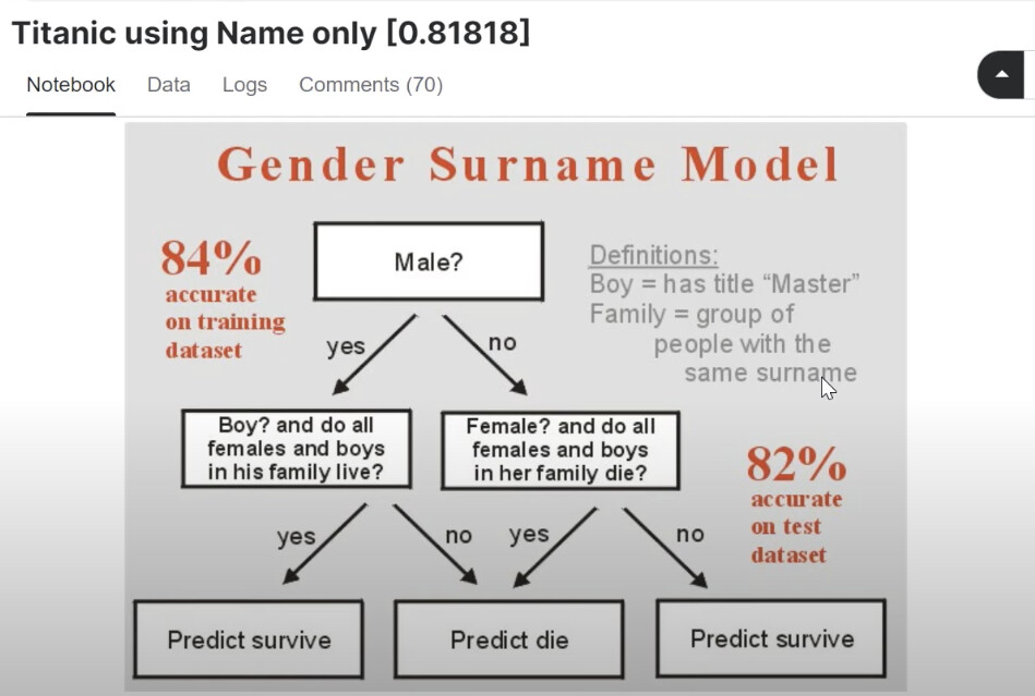
At the risk of stating the obvious, since we are we are talking about “Practical” ML. I’d like to point out one caveat regarding Chris’s Titanic using Name only [0.81818] notebook that survivorship of family members is likely not knowable at decision time. This is a form of a causality constraint. In addition I imagine most families would board a lifeboat together. While I know this a playground competition, I mention this as it comes up surprisingly often in practice. In the workplace you’ll be given lots of historical information and asked to create a predictive model. Without carefully considering the data generating process and when the variables are available you might find the most predictive variables are ones that violate this constraint.
Hi all, for anyone who wants to dive deeper into the “from-scratch” neural net we made in this lesson and learn each and every calculation involved in backpropagation, I highly recommend Andrej Karpathy’s The spelled-out intro to neural networks and backpropagation: building micrograd. It took me a couple days to get through the video, but it was well worth it to feel like I finally understood how backpropagation works! I hope it can help others as well.
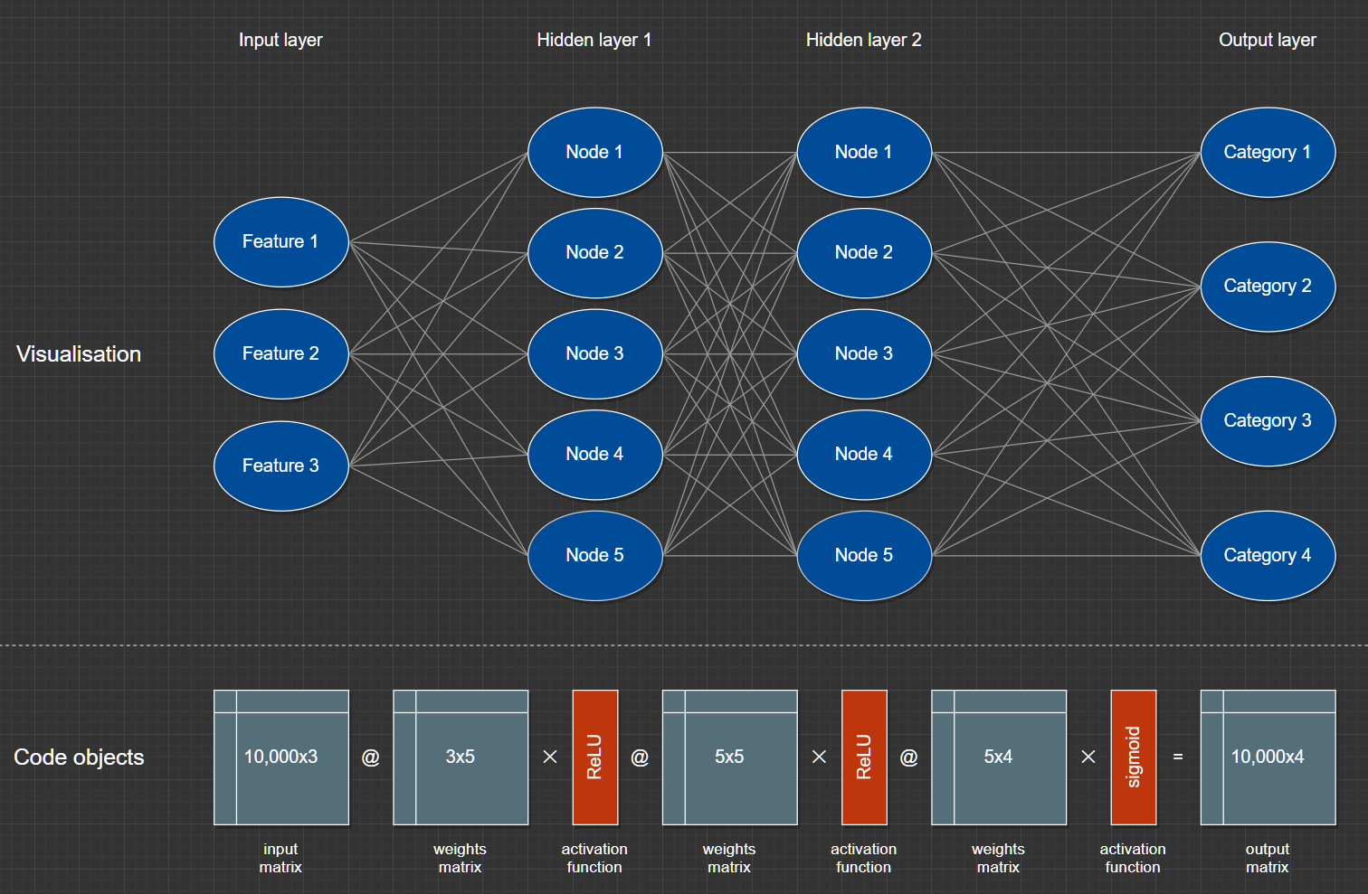
I tested out the implementation of a neural network from the video on the Titanic dataset and was pleased to see it work just as well/better than the Excel spreadsheet in reducing the final loss.
This is imagining a tabular dataset with 3 features, 10,000 rows, 2 hidden layers of 5 nodes each, classifying into 4 categories.
Disclaimers: it might not be right, I’m just learning; I’ve left out constants; it’s not really a straight multiply for ReLU and sigmoid, no softmax on the output.
The takeaway (for me at least) is that picturing a network as nodes and edges in layers isn’t particularly helpful and it’s probably best to just think in terms of the actual code objects, now that I know how it works. And they take a lot less time to draw