Neat !!
I have the same question. Have you find the solution?
Thanks.
Hi,
One observation in the last version of update() (see below) the Adam optimiser is initialised for every mini-batch. But Adam is a stateful optimiser, so by resetting it on every mini-batch, we are reducing significantly its performance. I moved line opt = optim.Adam(model.parameters(), lr) outside update() and achieved much faster convergence.
def update(x,y,lr):
    opt = optim.Adam(model.parameters(), lr)
    y_hat = model(x)
    loss = loss_func(y_hat, y)
    loss.backward()
    opt.step()
    opt.zero_grad()
    return loss.item()
from https://nbviewer.jupyter.org/github/fastai/course-v3/blob/master/nbs/dl1/lesson5-sgd-mnist.ipynb
That’s a good question !
When I implemented my home-cooked Adam optimizer class I naturally initialized it outside of the loop but did not compare it to initial Adam, I just went on implementing nn.Linear.
And when looking at the source code of Pytorch’s Adam I don’t see anything special that would justify it.
https://pytorch.org/docs/stable/_modules/torch/optim/adam.html#Adam
So it might be a mistake…
I finished the part where Jeremy talks about embeddings and it is really awesome. I googled some more information about it and seems easier for me to summarize embeddings as this:
- We can reduce the dimensionality of a categorical input vector (e.g. user and movie ids) by using embeddings.
- Similar categories are going to be close in the embedding space. I think that’s what Jeremy meant when he said that the dot product between User A and Movie B is going to be a high number if the user likes it and the movie is good. We could also see this on the example of german supermarkets.
Anyone know why when doing transfer learning the last layer is replaced by two layers? (instead of just a single layer with the correct dimensions for the new number of classes)
1 Like
By 2 layers, do you mean the sigmoid layer at the end as well ?
Hello All,
In Lesson 5, toward the end, Jeremy discusses the learning rate and momentum relationship for different batches in fit-one-cycle. Basically, “the learning rate starts really low and it increases about half the time, and then it decreases about half the time.”. In the other hand, every time our learning rate is small, our momentum is high and vice versa. He mentions that the reason is that when we are moving slowly in the beginning or the end we want to go faster; whereas when we are going faster (with higher learning rate), we don’t want to go too too fast. Basically, if you’re jumping really far, don’t like jump really far because it’s going to throw you off.
My question is, if we actually want to go slower in the middle, shouldn’t the momentum (I assume this is the beta) be higher (meaning we are considering more of the past points and give less weight to the current point)? What am I missing here?
Quote Jerermy: “We put two new weight matrices in there” In his picture, he has them separated by a Relu and followed by a sigmoid.
I.e. those two new layers do not include the sigmoid.
In case any one is interested, I have came up with a possible answer.
1 - in the beginning, we are in an unknown and potentially bumpy space. We want lower learning rate and a smoother and more focused (not faster, but more focused) trend to get out (hence, higher momentum)
2 - in the middle, we want to go faster and explore more freely. Hence, higher learning rate and lower momentum.
3 - in the end, we are close and do not want to jump around. Instead, slower and smoother progression toward the solution. Hence, back to lower learning rate and higher momentum.
1 Like
It’s a fastai thing. After your transfer learning ‘body’, Jeremy and co. found that it’s better to first add in an AdaptiveConcatPool layer, which is a MaxPool and an AvgPool, concatenated together. This ends up giving you 2x the activation count (from the ‘body’), which then gets back down to your desired number of classes via a couple of ‘Linear-ReLU-BatchNorm-Dropout’-type operations. The AdaptiveConcatPool and the other operations combine to form your ‘head’ of the model, so it’s two layers instead of the usual single layer that goes from the ‘head’ output to the desired number of classes.
You can call your learn.model, and it should show you how the layers get built, between ‘body’ and ‘head’.
Yijin
1 Like
What is a ‘unicode’ file as discussed in the lecture?
Hi,
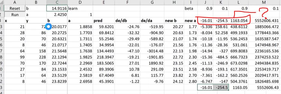
Firstly, apologies if my understanding is incorrect. Can anyone explain how S_0 is initialized in the below formula (mentioned in the video at 1:51:10) for gradient descent ?
S_t = alpha * gradients + (1-alpha) * S_t-1
What would be the values of S_0 in general ? In the lecture excel sheet, instructor Jermey has used some constants which I highlighted in the below screenshot. I am not sure how he has come up with the values at the first step (when calculating gradient step for the first time).
Most articles I referred to, explain the formula but not the initialization step. Would really appreciate if anyone can explain or refer some articles explaining the same.
Thank you.