Lesson 4 - Official Topic

[aditya.swami (Adi Swami)]

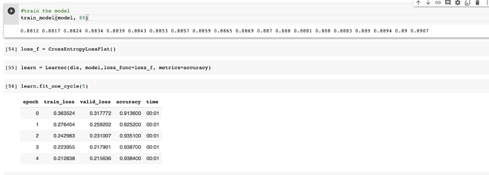
I tried it with CrossEntropyLossFlat and it trained to a higher accuracy in just 5 epochs which is amazing.
Thank you so much!

I really want to learn this foundational chapter very well before moving ahead because in some ways it feels like most things from here are optimisation tweaks to make training faster and/or with less data.

I am very new to programming and a lot of the programming side of things are confusing or feels like like magic. This forum has been such a help in getting me up to speed.

I’ll be reworking this notebook and try and build as many of these classes and functions from scratch to ensure it makes sense.

Thanks again!

[johannesstutz (Hannes)]

Perfect

I think your approach is great, creating all major functions from scratch and making sure to really get the basics right. I should do this more

And don’t worry about the coding, it will get easier. I had not written a single line of Python before this year and I’m feeling more comfortable every day. I can recommend freecodecamp.org and programiz.com for learning and codewars.com for some fun challenges.

Have fun

[PinkDraconian]

@PinkDraconian

So in short: Is there any way to get the image tensors from DataLoaders

@johannesstutz do you think you might be able to help me with this?

[johannesstutz (Hannes)]

Maybe You should be able to get the tensors just like this:

xs, ys = first(dls.train)

xs should be a tensor of for example the shape (64, 3, 224, 224) (batch size, channels, image size). Taking the mean over axis 0 gives you the average image in the batch.

You can write a loop over the dataloader like so:

for xs, ys in dls.train:
…

And create the averages for every class.

Good luck

[jimmiemunyi]

I solved the MNIST from scratch with the full dataset and my custom learner and loss function. If anyone is interested you can check out the notebook here:

Google Colaboratory

[mrfabulous1]

Hi immiemunyi hope your having jolly day.

I had a look at your notebook, great work, nicely written.
Cheers mrfabulous1

[meln1k (Nikita Melkozerov)]

Hello there,

In Chapter 4 in the section An End-to-End SGD Example we define a mean squared error function:

But what I noticed here is that our loss function turns out to be RMSE (because we take a square root in the end).

Is it a mistake in the code? All the following computations look like they were computed using the MSE and not RMSE.

[sua]

The function weights*pixels won’t be flexible enough—it is always equal to 0 when the pixels are equal to 0 (i.e., its intercept is 0).

I don’t really understand - what’s the intuition behind knowing that won’t be flexible enough. Also, why is it equal 0 and why would the pixels be 0?

[jimmiemunyi]

@sua

why would the pixels be 0

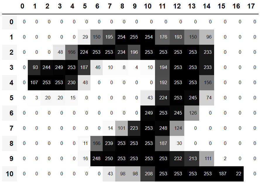
The Pixels would be 0 if the pixel represents a white color (in case of the black and white example we are using.) Remember when we printed out a portion of a sample 3 image and got this:

The pixels that are zero are white and the darkest ones are 255 or closer.

@sua

what’s the intuition behind knowing that won’t be flexible enough. Also, why is it equal 0

Each pixel will be assigned a weight associated with it. If the input (pixel) is zero, this function weight*pixel will always output a zero, since it is being multiplied with a zero. That’s why its not flexible enough since all the 0 pixels will have zero output. That is why we need a bias, to offset this value since the bias is added. weights*pixels + bias will sort out the issue of a zero pixel.

[sua]

Thanks for the response! Ok so that makes sense to me, however, I still don’t understand why do we not want 0? seems like that’s still helpful in our loss function? If a pixel is 0 in an eval set but a pixel has a nonnzero value in a test set, can’t we still calculate an error?

[jimmiemunyi]

@sua

I still don’t understand why do we not want 0

Here is a basic intuition why.

Let’s take one neuron for example. If the input to the neuron is zero, the neuron will output a 0. Alone, this is not a big issue, but it becomes a problem if this happens to this neuron for every one of the input samples (different images). Our images have a lot of pixels that are 0.

If this happens, this neuron will always produce 0 during the forward propagation, and then the gradient flowing through this neuron will forever be zero irrespective of the input.

In other words, the weights of this neuron will never be updated again. Such a neuron can be considered as a dead neuron, which is considered a kind of permanent “brain damage” in biological parlance

That’s my understanding. Maybe someone more knowledgeable can confirm this or give a better explanation.

[ACassoni (Alfonso)]

Hello! This chapter made me learn a lot

The only thing i am confused is in the following code line:
nn.Linear(28*28,30),
nn.ReLU(),
nn.Linear(30,1)

The “30” in the first line means 30 neurons (30 different models), so the first layer has 30 neurons and the second layer has 1 neuron (the output).

What if the first layer is “nn.Linear(28*28,1)” (like the model we trained before) instead of 30 and then pass through ReLU and then to another linear layer?

What is the purpose of the out_features parameter in nn.Linear? What does it do and why 30 or a number > 1?

[jimmiemunyi]

Hello

@ACassoni

The “30” in the first line means 30 neurons (30 different models),

Actually, the 30 stands for 30 different features. Giving the first layer 30 neurons means we are allowing our model to represent an image using 30 different features. This usually results in greater performance because each neuron learns a different set of weights to represent different functions over the input data.

That means that the first layer can construct 30 different features, each representing some different mix of pixels. You can change that 30 to anything you like, to make the model more or less complex.

[rypoll (Ryan Pollard)]

Hi all,

I am having trouble with the loss function and I’m wondering if anyone can help!

In notebook 5 there is a table that represents the probability of an image being a 3 or a 7:

|3|             7|  targ|idx|  loss|
|---|---|---|---|---|
|0.602469|0.397531|0|0|-0.602469|
|0.502065|0.497935|1|1|-0.497935|
|0.133188|0.866811|0|2|-0.133188|
|0.99664|0.00336017|1|3|-0.00336017|
|0.595949|0.404051|1|4|-0.404051|
|0.366118|0.633882|0|5|-0.366118|

Now from my interpretation the loss of predicting a 3, which is where an image has the target = 1, you take the probability of the image being a 7. So for the second row, the image is actually a 3, with a target = 1 and the loss is given by -Pr(7) = - 0.497935. This is the same as - ( 1 - Pr(3)).

We want to maximise this to get the best possible performance such that it should equal zero (maximise because it’s a negative number).
Or better to say, we want to minimise the probability that the model predicts 7 in this case, so we use SGD to find the parameters that minimise this.

My question arises from the multiclass case. The notebook says:

To see this, consider what would happen if we added an activation column for every digit (0 through 9), and then targ contained a number from 0 to 9. As long as the activation columns sum to 1 (as they will, if we use softmax), then we’ll have a loss function that shows how well we’re predicting each digit. We’re only picking the loss from the column containing the correct label. We don’t need to consider the other columns, because by the definition of softmax, they add up to 1 minus the activation corresponding to the correct label. Therefore, making the activation for the correct label as high as possible must mean we’re also decreasing the activations of the remaining columns.

I interpret this like this. If we have numbers 1 - 9, with the image inputted being an actual 3, we use the result of the softmax which gives the probability of it being 3 (and of course the probability of being all the other numbers) as the loss function. Therefore we’re looking to maximise this value, and hence minimise 1 - Pr(3). My question is, is this loss function, in my example explained here, 1 - Pr(image = 3)? There’s no mentioned of 1 - Pr(3) in the notebook, well the 1 - operation in general, so that is confusing me!

Thanks!

[BrownJenkin]

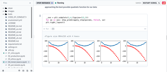
Possible bug! I have loaded the Paperspace + Fast.AI notebook on https://console.paperspace.com/ and ran all of the cells in the full book ipynb file. I get this, which means something went very wrong somewhere:

I did not change any of the default settings when creating the notebook. All the notebook cells are unchanged.

Many thanks!

[jimmiemunyi]

Try a higher learning rate

[BrownJenkin]

Thank you! I can see change when running this cell for the first time, but a different problem arises when I run it several times more:

It seems to be stuck on these three parameters:

tensor([ 0.1753, -0.6854,  1.3738], requires_grad=True)

When looking at the speed variable initialisation:

speed = torch.randn(20)*3 + 0.75*(time-9.5)**2 + 1

Ignoring the added randn noise, I find the parameters (please correct me if I made an error. I am error prone):

0.75 * (time - 9.5)**2 + 1 =
= 0.75 * (time**2 -19 * time +90.25) + 1
= 0.75 * time**2 -14.25 * time + 68.5

so the underlying parameters (if I did not make any errors) are a = 0.75, b = -14.25, and c = 68.5 which are different from the inferred a = 0.1753, b = -0.6854, and c = 1.3738.

Also, I expected the embedded outputs shown in the notebooks to be the same as the outputs after one runs the unchanged notebooks top to bottom for themselves. Without having working code and expected output great confusion arises. I have written an issue https://github.com/fastai/fastbook/issues/500 concerning this problem.

[BrownJenkin]

Actually, the inferred points of the embedded output seem to be reaching the same values as the inferred points of my output.

I am still confused. Why do they not converge?

[matdmiller (Mat M)]

The main point of this section of the book/notebook is to demonstrate how SGD works so you understand the concept. It shows you that after running several epocs the parameters are improving which demonstrates it’s working. At the end of running this you should not expect the learned parameters to exactly match the values used in the original equation exactly, just that they are closer to them after training than the random ones that were generated.

In the example in the book, it is impossible to achieve perfect convergence because parameters in the quadratic equation do not exactly match the parameters in the example speed equation (ex: a*time**2 vs 0.75 * (time - 9.5)**2 : parameter for 9.5 is missing).

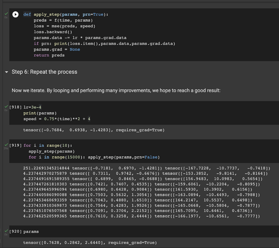
If you want to see the learned parameters converging much closer to the factors in the speed equation you can remove the noise and change the factors in the speed equation so they match the quadratic equation (ex: speed = 0.75*(time)**2 + 4). I then added additional items to the print statement in the apply_step function if prn: print(loss.item(),params.data,params.grad.data) and move the print statement above the param.grad = None line so you can easily see the parameters changing. The last thing you can do is play around with increasing the learning rate (if you go too high, it will not converge so change it slowly) and apply a lot more iterations. You will also need to run more iterations for the values to converge. See screenshot.

There are a lot of tricks for improvements all around which are discussed later in the course. The main thing is just having a basic concept of how SGD works.

[olliebeannnn (Ollie Khakwani)]

In the example though, it seems like the bias is being added to the entire image, not to individual pixels? I could be missing something though