In the 4th chapter of the book, it is stated that there is no difference between models with two large layers versus models with multiple smaller layers, with the latter being easier to compute.
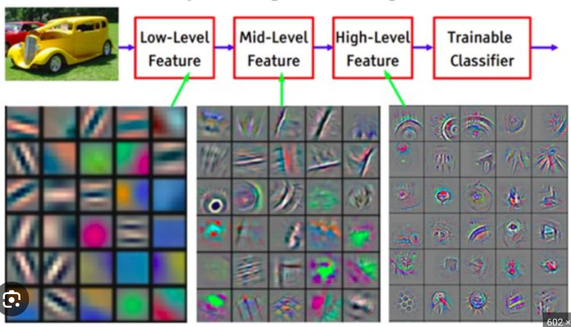
However, this reminded me of the multi-layered image classifier that Jeremy presented. It was demonstrated that the first layer identifies simple shapes, and the subsequent layers, building upon the previous ones, recognize increasingly complex features.
Doesn’t this contradict the thesis presented in the book? I mean, if there are only two large layers, there cannot be such a hierarchy of feature recognition, as nodes within the same layer are not connected to each other.
I managed to replicate the training process from scratch on a new notebook without adding these extra dimensions and it seems unintuitive to me why it has been done so.
I also came across https://minitorch.github.io where you get to build your own mini PyTorch library from scratch. I’m looking forward to do it once I’m through with Part 1.
I also came across https://minitorch.github.io 1 where you get to build your own mini PyTorch library from scratch. I’m looking forward to do it once I’m through with Part 1.
Part 2 of the fastai Course also involves you recreating many of PyTorch’s functions from scratch.
I feel a little silly for asking, but what is the assignment for Lesson 3? I see some people discussing working with the MNIST dataset, but I can’t find any prompt or instructions to go off of.
Also, should we be sharing our work for each lesson here, or on the lesson thread, or maybe another place?
To answer your first question: there is a “Further Research” section after each chapter (see the chapter notebook) which has prompts for us students to explore.
For lesson 3/chapter 4, the prompts are:
Create your own implementation of Learner from scratch, based on the training loop shown in this chapter.
Complete all the steps in this chapter using the full MNIST datasets (that is, for all digits, not just 3s and 7s). This is a significant project and will take you quite a bit of time to complete! You’ll need to do some of your own research to figure out how to overcome some obstacles you’ll meet on the way.
I guess my confusion is that for Lesson 1 the video and notebook explicitly state the homework, which is different from the textbook. Then Lesson 2 is all about publishing a model, so the assignment (to create and publish a model) seems obvious, though I can’t find where it was explicitly stated. For comparison, the lesson 2 textbook assignment is to write a blog post (among other things).
After reviewing the Lesson 3 video it does appear to suggest homework. I believe it is referring to this kaggle notebook, but I don’t see a clear link there in the Lesson 3 resources. This again is different than the suggested homework from the textbook assignment, which you’ve kindly pointed me to.
So all that is to say, it is easy enough to follow the textbook. However the videos suggest that the material from the videos is different from the text and that one of the assignments for each video lesson is to read the corresponding chapter in the textbook. And given that the first 2 lessons appeared to assignments that were different from the textbook, it seems strange to pivot there for Lesson 3.
Maybe I am over thinking this ¯_(ツ)_/¯
I guess doing “all the things” will be best for learning.
Ah I see. Yeah what I did in response to that segment of the video is run each cell in the “Getting started with NLP for absolute beginners” notebook before the Lesson 4 video. You are right that the material in the videos doesn’t always match the textbook, and I too took the “doing all the things” approach to cover it all.
Hi all: I have a question regarding using spreadsheet to create a machine learning model. I don’t understand how creating the Ones column with the value of 1 can replace the value of b, the constant, in this forumua, mx + b. Can someone please explain it to me? thanks!
From what I understand, the Const weight (highlighted below) is the actual b bias value in your mx + b representation, and the Ones column is there so that the Const bias is added during matrix multiplication (SUMPRODUCT in Excel) of the data (Table13[@[SibSp]:[Ones]]) and the weights ($R$4:$AA$4).
I really liked Jeremy’s example of an infinitely complex function in the video here https://www.youtube.com/watch?v=hBBOjCiFcuo&t=2717s, but was a bit thrown at first by having y = ax + b within the relu definition. My understanding is the ReLU operation is just the max(0, y). I then got confused by the absence of the b in the titanic example. Once I realized relu was the max(0, y), the operations made more sense to me:
the multiplication is the ax + ...nx part of the equation,
the multiplication by the ones gives you the b,
then you max(0,y) the result.
Also a big thank you to Jeremy for separating all this math from convolutional neural network structures. Most previous stuff I’ve read online jumps into convolutions straight away, which made the math much harder to follow. I’m glad this course saves convolutions for the final week!
I have a question related to calculating the gradients. In the section of Calculating Gradients, it was shown that loss function was a function of parameters, and thus I was able to connect for how to calculate slope wrt a single parameter. But in the section of An End-to-End SGD Example, where the loss function = ((preds-targets)**2).mean(), I can see that apart from depending upon the parameters/weights, loss function will also depend upon time, then how will the slope/derivative will be calculated?
Hello everyone, I have a doubt regarding the NN model for the titanic dataset created during the video lesson.
To compute the predictions from the model, we do ReLU(X @ W1) + ReLU(X @ W2).
Since we don’t use the result of the multiplication for W1 as the input of the multiplication for W2, is it correct to say that this is a NN with 1 layer?
From what I knew before the course, if this was to be considered a NN with 2 layers, I would’ve expected the predictions to be calculated with ReLU(Relu(X @ W1) @ W2).
If this can be considered a 1 layer NN, my intuition would be that the parameters in W2 would end up being the same as the ones in W1 (outside of difference due to random initialization) since they are connected by the same function to the inputs, is that wrong?
If not, what justifies the improved performance that we obtain with the second set of parameters?
I have a question related to the paragraph given below in the section The MNIST Loss Function
The loss function receives not the images themselves, but the predictions from the model. Let’s make one argument, prds, of values between 0 and 1, where each value is the prediction that an image is a 3. It is a vector (i.e., a rank-1 tensor), indexed over the images.
The purpose of the loss function is to measure the difference between predicted values and the true values — that is, the targets (aka labels). Let’s make another argument, trgts, with values of 0 or 1 which tells whether an image actually is a 3 or not. It is also a vector (i.e., another rank-1 tensor), indexed over the images.
So, for instance, suppose we had three images which we knew were a 3, a 7, and a 3. And suppose our model predicted with high confidence (0.9) that the first was a 3, with slight confidence (0.4) that the second was a 7, and with fair confidence (0.2), but incorrectly, that the last was a 7. This would mean our loss function would receive these values as its inputs:
trgts = tensor([1,0,1])
prds = tensor([0.9, 0.4, 0.2])
Question - At one point it is said Let's make one argument, prds, of values between 0 and 1, where each value is the prediction that an image is a 3, then shouldn’t the last line of the paragraph denoting confidence as (0.9, 0.4, 0.2) should all denote the confidence for the digit 3, rather than sometimes the confidence for 3 and sometimes for 7?
Here’s my understanding of it: the interpretation of the predictions is based 1.0 being a fully confident prediction for a 3, and 0.0 being a fully confident prediction of 7, aka binary classification.
Anything above 0.5 shows confidence towards a 3, and anything below 0.5 shows confidence towards a 7.
prds = tensor([0.9, 0.4, 0.2])
0.9 is greater than 0.5 and is very close to 1.0 so it’s a highly confident prediction of 3.
0.2 is less than 0.5 and is pretty close to 0.0 so it’s a fairly confident prediction of 7.
0.4 is less than 0.5 and is slightly closer to 0.0 than it is to 1.0 so it’s a slightly confident prediction of 7.
One thing to note is that the selection of 0.5 as being the threshold between the two classes is arbitrary. Let’s say you wanted the model to predict 3s only if it was very confident that the image was a 3. In that case we might have the threshold that divides “is a 3” and “is a 7” as something like 0.95. Then, none of the predictions would count a prediction for a 3.
(i misused convolutional here, what I meant was the way in which features feed-forward in deep learning, which i’d often seen communicated with a complicated diagram and lots of math i didn’t understand. showing a single layer with 2 features + bias before scaling up really helped me grok this.)
Hi Kamui, thank you for sharing this video that I’ll watch. But there is something I don’t intuitively get. In Jeremy’s notebook we obtain a gradient for each weight (a, b, c). But isn’t the value of a gradient also depending on x? I mean, we calculate a gradient at a certain position, right? So let’s imagine we have 10 values for x, I would expect a 10 gradients for a, 10 for b and 10 for c…
@mastronaut The gradient is usually computed with respect to the loss function. And that is a single value because it is a mean (or sum) of the loss of all examples x. That’s why you only get one gradient per parameter. Actually, I don’t think pytorch even allows to have multiple grad values per parameter.
I also recommend watching the micrograd video from Karpathy as it shows each step of this process.