thanks!
1 Like
Hi Everyone!
After watching the lesson 3 video, I am stuck on chapter 4 of the notebook, and I was hoping someone could help me out!
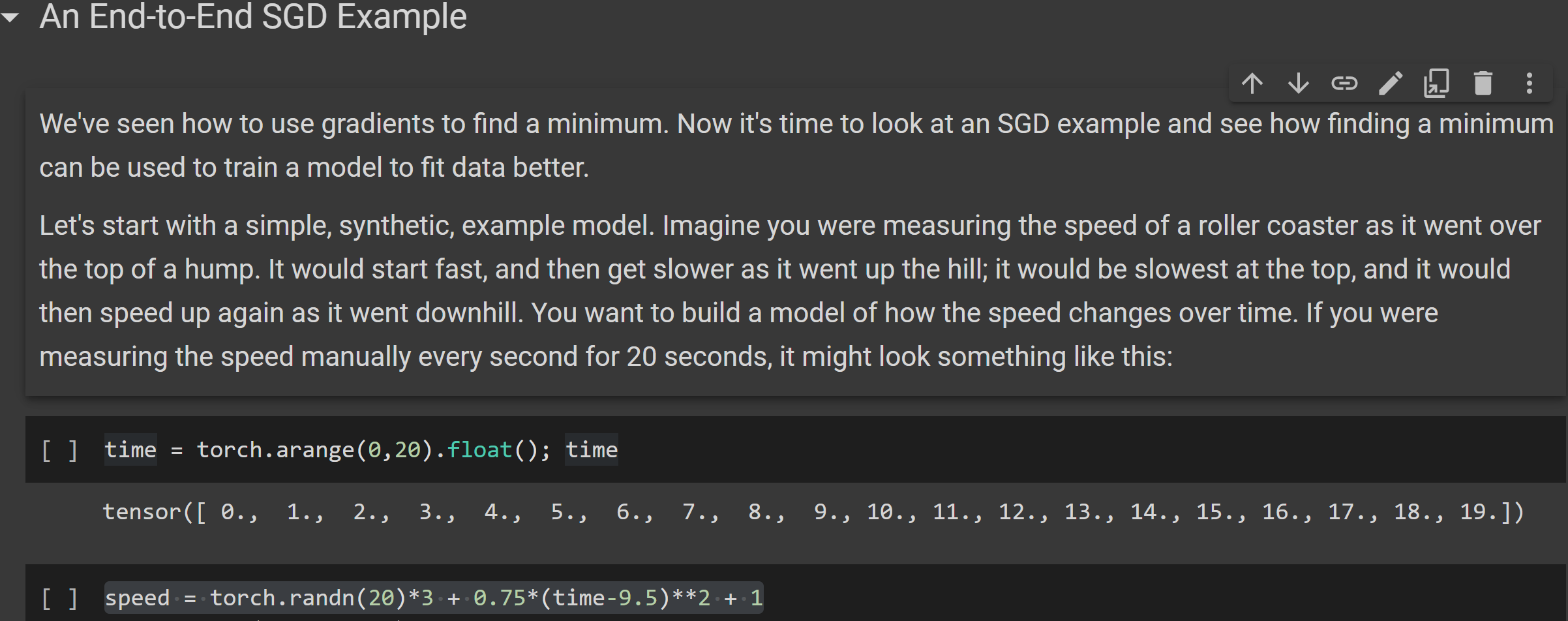
I am doing the “End to End SGD Example” part of chapter 4.
Can someone tell me why the ‘speed’ variable has been assigned with the following formula: “torch.randn(20)3 + 0.75(time-9.5)**2 + 1”? - Why are we using this specific formula in this specific manner? Is this formula supposed to be similar to a quadratic equation? Why are we subtracting ‘9.5’ from the ‘time’ variable in this formula?
I have attached a relevant screenshot as well.
I am trying to use Gradient Notebook on Paperspace.
This is my first time, and I just simply created an account (didn’t link any of my credit card).
But whenever I select Paperspace + Fast.AI, I don’t see any available machine, even the free one.
Do I need to at least update payment method in my account to use the free machine?

@jeremy should the HuggingFace Spaces Pets repository listed here be in the resources for Lesson 2 instead? Lesson 2 (and chapter 2 of the book) seem more related to pet classification than Lesson 3.
Checkout https://www.learnpytorch.io and the official get started page in PyTorch
1 Like
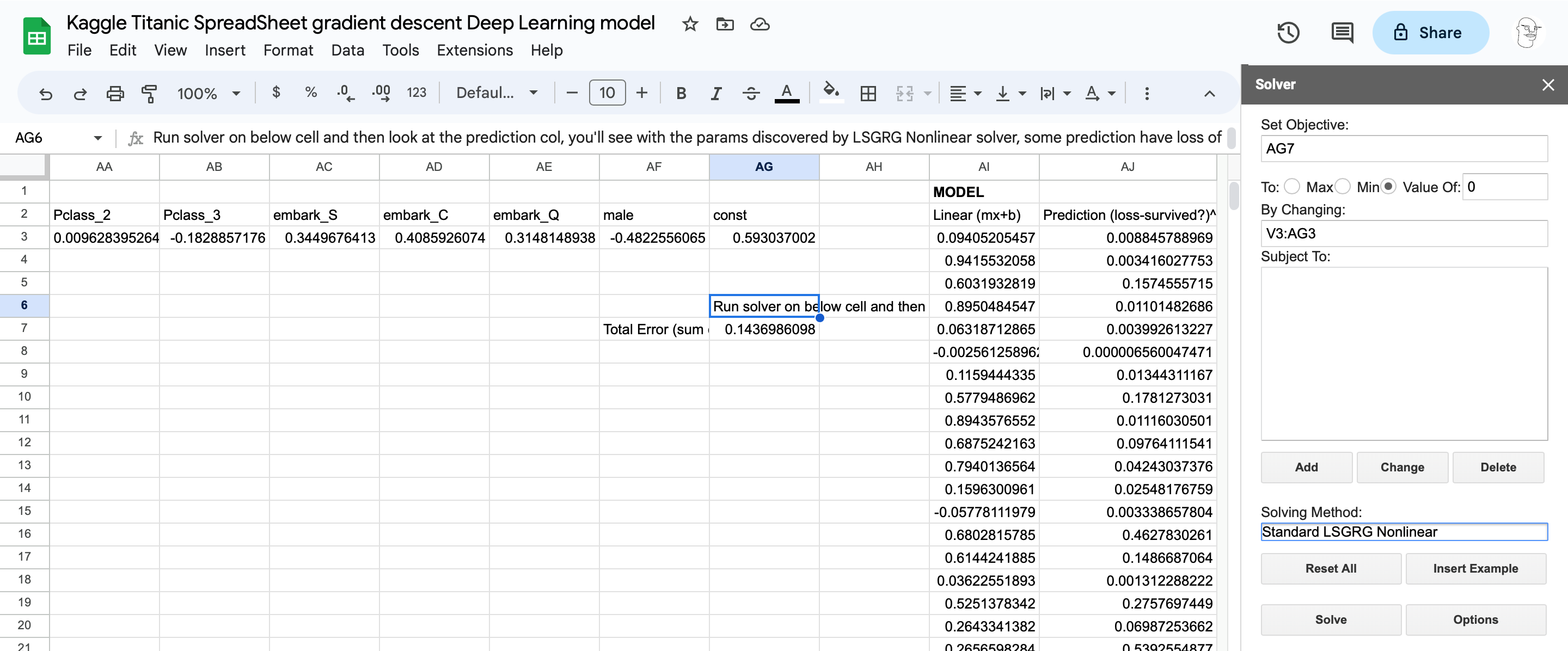
Google Sheets solution - lesson 3.
Results
The solver plugin required to get this working in Google Sheets is a bit limited, however you’ll see it was able to make accurate predictions (Loss of 0.00) for a number of passengers after a few iterations.
Note:
- Google Sheets doesn’t have a native solver and requires the solver plugin be installed:
- Settings for the solver look like this:
This is an aspect that I was also confused by.
Using the example given in lesson 3 of finding the quadratic ax^2 + bx +c that best fits the “noisy” dataset.
I’ve been thinking of it like this.
- We have a noisy plot, this is our “dataset”,
- We plot an arbitrary quadratic, with initial values for params a,b,c on the same graph, calling this the prediction:
y_pred = ax² + bx + c - For each point in our dataset we calculate the “loss”, i.e. distance of this point to the corresponding point on the quadratic (corresponding here means, the points we’re measuring the distance between have the same x value, another name for the x variable here is “the independent variable”) that we just drew.
loss = y_pred - y_actual
- We then find the mean of all these losses.
MSE = 1/n * Σ (y_pred - y_true)²
Expanding out the y_pred - y_true part of this (i.e. the loss e, without the mean square part), we can see our parameters within this loss function like this:
e = y_pred - y_true = ax² + bx + c - y_true
Our MSE can now be written as:
MSE = 1/n * Σ e²
-
So at this point we have a mean, which involves all our parameters (a,b and c) but we want to see how this loss changes with respect to just one of these parameters, let’s say
b. Asbchanges the loss will change, so I’m guessing under the hood we do this for a few values of b (would love to confirm this), this gives us datapoints to draw another plot, this time ofbon the x-axis and MSE on the y-axis. The gradient of this line at the current value of param b is the gradient we want to calculate. Which we do, as you mention using the gradient of the tangent to the line at that point, aka, “the derivative” or∂MSE/∂b. -
If this gradient
∂MSE/∂b, which is called the derivative of MSE with respect tobis positive we know we want to decreaseb, and vice versa for the next layer of our model.
Hope I am correct in all that and it makes sense. I realize there are some chain rule derivations that can be done on MSE = 1/n * Σ e² to express all this mathematically but I am not comfortable with the chain rule right now.
1 Like
That reasoning makes sense to me. I view the MSE as a function defined on the a,b,c axes and and the gradients of MSE with respect to each variable a,b,c are used to move in the direction of the minimum of the function.
I had one question for the process of using gradients to reduce the MSE(cost). If we find the gradient and adjust the value of the variable to cause the MSE to decrease isn’t it possible that we move our solution into a direction that is not towards the true minimum? For example in the image below the gradient from the current location leads to a lower MSE but this movement is in the opposite direction of the true minimum value of the MSE.
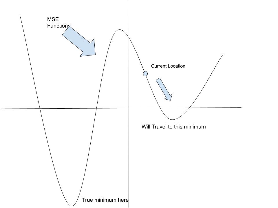
Am I missing something in my understanding here?
1 Like
That is an actual issue; I’m not too aware of the methods there are that can overcome this, though I assume the fastai Learner class has optimizers that have algorithms built in to overcome this.
But this issue is why there can be a lot of variation when training a model: sometimes you begin at a more favorable location in the optimization landscape, and other times you don’t. Luck can play a factor.
Some extra information you may be interested in.
The method you describe is known as “Greedy Search”. It only optimizes for short-term gain. It ignores any negative changes and accepts only positive changes. So it’s very easy to get stuck in a local optimum with this method.
One method of overcoming this is known as “Simulated Annealing”. You have a value that’s known as the temperature. The higher the temperature, the more likely it is that a negative change will be accepted. During the early stages of training, the temperature is very high, meaning either a negative or positive change is accepted. As training progresses, the temperature gradually decreases and so the chances of accepting a negative change decrease.
The probability whether a negative change is accepted is defined by the following formula.
e^{-\frac{S_{\text{old}} - S_{\text{new}}}{T}}
S_{\text{old}} is the old score/loss/cost, S_{\text{new}} is the new score/loss/cost, and T is the temperature.
1 Like
Thanks! That makes sense. The simulated annealing thing is also very interesting and it seems a little similar to decaying learning rate talked about in lecture – both restrict movement as we move closer to a solution.
Yes, I suppose that is one way to create a decaying learning rate — haven’t really thought of it like that heh.
1 Like
Suhaas, I had the same question, this is what I figured out.
If you use Stochastic Gradient Descent, instead of vanilla Gradient Descent (which is plotted using the entire dataset for a given independent variable), SGD uses random subsets (mini batches) of the data to calculate the loss for a given value of the independent variable, this randomness this can help jump out of shallow local minima.
- These are called Noise Induced Jumps Using mini-batches causes this “noise” or “vibration” in the gradient - as we change the independent variable, the gradient is going to be inconsistent - and may on occasion reverse the gradient direction, which would result in us escaping the local minima.
- Probably not a very helpful analogy but - imagine if there was a ball bearing rolling around your diagram, imagine plucking the plot like a guitar string, this would help it jump out of a local minima and it’d eventually find the global minima.
- Mini batches also mean the parameters are updated more frequently - basically I think it means we can calculate the loss multiple times for each independent variable, taking an ‘average’ gradient or similar.
That said, SGD isn’t guaranteed to find the global minima for non-convex loss functions.
But even with this limitation It’s worth noting that other variables that are probably worth thinking about… particularly as there are a lot of variables at play and the model is working in high dimensionality. Off the top of my head, these could work, and are likely already part of the model development workflow.
- Using Ensembling to mitigate one model that’s stuck in the local minima.
- Tweaking learning rate.
Finally, I’ve read that in practice people don’t worry a great deal about this because in practice a local-minima isn’t strictly a bad thing, and often doesn’t result in significantly different accuracy. Basically there are Many Equivalent Solutions
In a neural network with many layers and many neurons per layer, there are often many different combinations of parameters that produce equivalent or nearly equivalent results. This means that even if you find a different minimum each time you run the training algorithm, the practical differences between these solutions may be negligible.
2 Likes
Complete beginner here without a ComSci background. I just finished going through Chapter 4 of the book after watching Lesson 3 and doing the other notebooks. It took me 3 days and it was HARD. I get that its basically the same thing as Lesson 3 but Chapter 4 dived really really really deep into the nitty gritty and most of that just went over my head.
My question is, is it alright to continue the course. Would it be better to come back to this Chapter later or nail this down now before moving forward?
I struggle with all the manual code in Chapter 4 (rewriting even a third of the code would be a huge effort and even thinking of attempting the 2 task under “further research” is intimidating) but able to answer at least 60-70% of the questions at the end.
1 Like
Jeremy advises that in order to do the course you must have at least one year of coding experience. That way you won’t find code and coding concepts hard to grasp. I advise you go learn Python and do some small projects with it for a while then come back to the course. As for the chapters you don’t have to nail things down from the first time. You can learn by doing multiple passes of the course: in the first one you get just the general ideas, in the second you go deeper etc…
Have fun!
3 Likes
You a correct, for this simplistic 2D exmaple, you may get stuck at the local minimum. But consider real problems are multidimensional. Consider the example image is a cros-section from a 3D world, with the middle peak being the top of a hill. Water will flow from the local minimum, around the back of the hill into the “true minimum”.
Now of course the 3D would has local-minima-pits you could get stuck, but consider real world problems are multi-dimensional, and mostly you can escape a pit though one of those dimensions. The corallary is, the more independent dimensions in your training data, the less likely you’ll get stuck in a local minimum.
1 Like
Hello all!
I am working through the How does a neural net really work? notebook. To better understand the concept of gradient descent, I tried to build a simple example:
import torch

# Create a simple computational graph
x = torch.tensor([2.0], requires_grad=True)
y_true = torch.tensor([9.0])

# Compute the predicted output
y_pred = x ** 2

# Compute the mean squared error (MSE) loss
loss = ((y_pred - y_true) ** 2).mean()

# Perform backpropagation and compute gradients
print("loss")
print(loss)
loss.backward()

# Access the gradients of x
print(x.grad)
lr = 0.1
x = x- lr * x.grad
x
The outputs for this program are
loss
tensor(25., grad_fn=<MeanBackward0>)
tensor([-40.])
tensor([6.], grad_fn=<SubBackward0>)
As I understand it, the recommended next numbers to test is 6
If I go back then and swap out 6 in the X tensor: x = torch.tensor([6.0], requires_grad=True) and run it again, I suddenly get a crazy result the next time round.
loss
tensor(729., grad_fn=<MeanBackward0>)
tensor([648.])
tensor([-58.8000], grad_fn=<SubBackward0>)
Now it seems like its telling me to use -58.8 as the next value for X. If I follow that step in 2 more cycles the recommended x value becomes an infinitely long number
What am I doing wrong here?
I think after you replicated the notebook from scratch you should find a dataset, which is similar and try to apply what you have learned there
I would suggest that you try to first understand whaat is going on with things before you move, otherwise you might confuse yourself in the process. if you are confused the best place to ask is the forums
Hello all, I am trying to build my own automated gradient descent and running into some challenges:
This is my program:
import torch

x1 = torch.tensor([1.0], requires_grad=True)
y_true = torch.tensor([9.0])

def calculate_loss(x1):
    y_pred = x1 ** 2
    return ((y_pred - y_true) ** 2).mean()

for i in range(30):
    loss = calculate_loss(x1)
    loss.backward()
    with torch.no_grad(): x1 -= x1.grad*0.01
    print(f'step={i}; loss={loss:.2f}; x={x1}')
It gives the following results
step=0; loss=64.00; x=tensor([1.3200], requires_grad=True)
step=1; loss=52.67; x=tensor([2.0232], requires_grad=True)
step=2; loss=24.08; x=tensor([3.1235], requires_grad=True)
step=3; loss=0.57; x=tensor([4.1293], requires_grad=True)
step=4; loss=64.82; x=tensor([3.8053], requires_grad=True)
step=5; loss=30.03; x=tensor([2.6471], requires_grad=True)
step=6; loss=3.97; x=tensor([1.7000], requires_grad=True)
step=7; loss=37.33; x=tensor([1.1683], requires_grad=True)
step=8; loss=58.30; x=tensor([0.9934], requires_grad=True)
step=9; loss=64.21; x=tensor([1.1369], requires_grad=True)
step=10; loss=59.40; x=tensor([1.6309], requires_grad=True)
step=11; loss=40.20; x=tensor([2.5386], requires_grad=True)
step=12; loss=6.53; x=tensor([3.7057], requires_grad=True)
step=13; loss=22.39; x=tensor([4.1714], requires_grad=True)
step=14; loss=70.57; x=tensor([3.2354], requires_grad=True)
step=15; loss=2.15; x=tensor([2.1095], requires_grad=True)
step=16; loss=20.70; x=tensor([1.3674], requires_grad=True)
step=17; loss=50.84; x=tensor([1.0154], requires_grad=True)
step=18; loss=63.50; x=tensor([0.9871], requires_grad=True)
step=19; loss=64.41; x=tensor([1.2756], requires_grad=True)
step=20; loss=54.36; x=tensor([1.9403], requires_grad=True)
step=21; loss=27.41; x=tensor([3.0114], requires_grad=True)
step=22; loss=0.00; x=tensor([4.0742], requires_grad=True)
step=23; loss=57.74; x=tensor([3.8986], requires_grad=True)
step=24; loss=38.43; x=tensor([2.7563], requires_grad=True)
step=25; loss=1.97; x=tensor([1.7687], requires_grad=True)
step=26; loss=34.48; x=tensor([1.1965], requires_grad=True)
step=27; loss=57.28; x=tensor([0.9864], requires_grad=True)
step=28; loss=64.43; x=tensor([1.0931], requires_grad=True)
step=29; loss=60.92; x=tensor([1.5411], requires_grad=True)
The program never seems to find its way consistently to the right answer of 3
1 Like