Thanks Vikrant
Does “Once through the loop” == Process a mini batch?
Thanks Vikrant
Does “Once through the loop” == Process a mini batch?
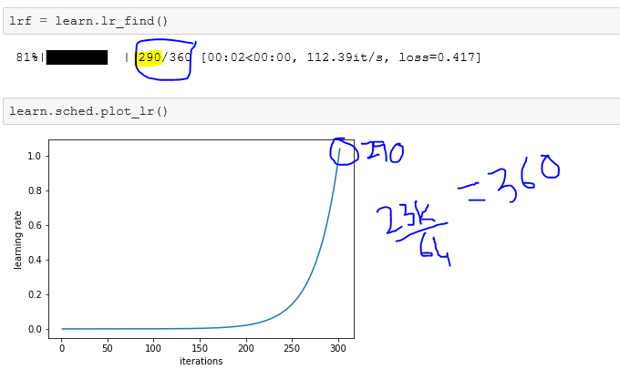
For 23k records, we’ve 64 batch size. Mathematics kicks in:
23k/64 ~= 360. So, loop 360 times. So, once in a loop is one mini batch.
Note: This is my understanding.
Awesome explanation - thanks! 
But to follow up - changing vs resetting learning rate…
Does change the learning rate after every mini match mean move it towards a smaller increment, after beginning at its maximum value for the first batch?
Does resetting the learning rate mean swapping the maximum starting value for another one? If so, would this only make sense when we have unlocked the model and are applying different rates to the various layer groups?
It’s because lr_find stops the training loop early, as soon as the loss gets significantly worse. I think it is showing a bug in tqdm that it’s reusing some object, but I’m not sure of the details…
So, I went ahead and used 0.001 instead of 0.01 until differential learning rate step (@jeremy, per the previous discussion I used 0.01 from lecture)
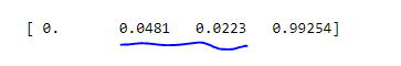
Trying to understand loss for the validation set. Below summary is with precompute = True
0.0223/0.0481 ~= 46%. Do I read validation loss as half of learning loss? @tensoralex thanks!
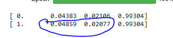
Assuming we read validation loss in terms of training loss, the validation loss after enabling augmentation has reduced from 46% to 42%. So, 4% improvement?
0.02077/0.04859/ ~= 42%
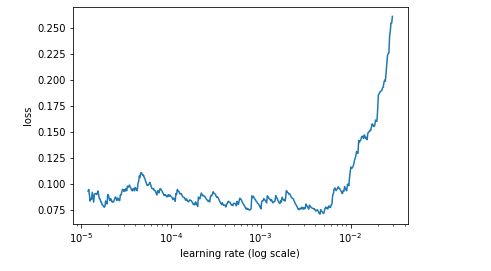
After unfreezing my lr finder shows that ~0.01 is optimal lr?
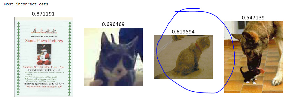
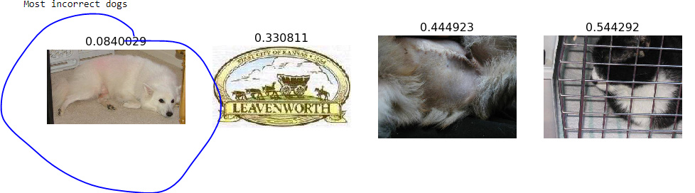
Overall accuracy is 99.6 with 8 wrong predictions. I’m curious to understand the factor(s) that would have confused learner for the highlighted case. It gave .61 probability that it’s dog against .39 of being a cat.
Also what confused it for dog case? Is it the carpet? The probability of being a cat is huge, 0.92.
Actually It seems you have training loss (0.0481) ~2 times higher than validation loss (0.0223).
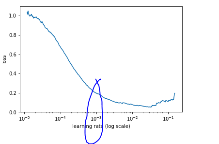
not to worry about ‘lr’ finder, I tried and plot suggest an optimal lr of 0.001
if I recall lecture correctly, Jeremy picks the order of magnitude where min loss belongs to, so it should be 0.01 according to first and second graphs.
I tried to implement what we learnt so-far on Kaggle statoil image data (ship or iceberg). In case, some one wants a head start for that competition, here is the link.
https://www.kaggle.com/grroverpr/cnn-using-fastai-lb-0-2094/
Thank you. I updated the original question.
Hi, @vikbehal
I don’t know if our understanding of lr_find() is the same.
Let me state my understanding first.
lr_find() schedule a learning_rate trials from min_lr (1e-5 by default) upto max_lr (10 by default).
A constant factor “mult” is computed according to min_lr, max_lr and number of batches.
After every batch, the learning_rate is multiplied by “mult”. (so in linear scale, the data points are evenly distributed). Or, in other words, learning_rate at i-th batch is equal to min_lr * mult ^ i.
The y-axis (loss) is the loss for the corresponding batch.
(I think the corresponding source code is in “learner.py” and “sgdr.py”. )
There are two interesting things. For an untrained model, the initial loss is definitely very large. Since the learning rate at the beginning trial is very small, we almost sure we will get the high loss and we can only change the parameters in the model slightly.
The second thing is that, larger learning rate will reduce the training time and lower learning rate helps to find lower loss. The most common practice usually choose a relatively large learning rate at the beginning and reduce it later to improve accuracy. Picking the learning rate is a trade-off between computation time and accuracy.
You probably already know all of these. Sorry to restate them.
Get back to your question.
To me, it seems we should use 1E-3 or anything between 1E-3 and 1E-4 should do.
The difference from using 1E-2 should be training time rather than accuracy.
(will you give a try?)
It seems to me that the model is already well-trained.
The change of loss seems caused by the variation of mini batches.
A more rigorous test is to compare the mean and std.dev. of the loss between this and the model (without backprop) .
This is just my opinions, which might not be correct.
Please let me know what you think.
Everything you said sounds just right! But I just wanted to comment on the last sentence above - using a higher learning rate, along with SGDR, can improve accuracy, since it can “jump out” of spiky parts of the loss function surface.
Does fastai’s AWS AMI provide ‘planet’ data as well or we should be downloading it?
This is for lecture 2
My data directory on AWS has only ‘dogscats’ subdirectory.
Note: Tried searching this thread but couldn’t find.
The AWS AMI only has dogscats, so you’ll need to download anything else you work on.
Hi, @jeremy
Thank you for pointing it out.
You are absolutely right.
The idea of “stableness” or “resilience” of an optimum point quite opened my mind.
( very similar to the width of potential well in physics. )
I think the narrow width also some how relates to the “over-fitting” problem,
and seeking a more “resilient” optimum point is actually moderating the over-fitting problem.
Just like you said (and I paraphrased here), given a different set of unseen data points, we want all of them contained by this “potential well”.
I wonder if we can define a loss function that takes the resilience into account.
But for now, greater learning rate definitely helps.
BTW, thank you for introducing the cosin annealing with restart. I think it is super cool. 
Glad to be helpful! A direct measure of ‘resilience’ would certainly be an interesting research direction, especially if it’s differentiable.
This is looking very good - you may want to add a note that you’re doing the in-person course, that’ll be released at the end of the year; otherwise people might be confused!
BTW, you might find dn121 a better architecture for this. If you try it, I’d be interested to hear how it goes.
Thanks @jeremy. Sure, I will mention that in there. I am thinking to keep on updating the code after each week’s DL class and implement whatever we learn. I will explore dn121 and let you know. Thanks
In Lesson-2 @jeremy mentioned that one way to do data augmentation in NLP is using synonyms
from what @Ray2 said, many things went overhead due to mathematical terms but I believe choosing ‘lr’ in itself is a skill which depends on many factors. An important note is to look at current model’s accuracy, consider bit higher ‘lr’ to avoid spiky parts.
@jeremy so there is no thumb rule while choosing lr in initial stages? 
Start with an optimal value (e. g. found through lr finder) and decrease it gradually in every iteration.
Resetting it to default optimal value is something that is to avoid spiky parts. When do we reset is a question of our experience?..in lectures until now we’ve reset it after every cycle. A cycle length varies and depends upon how many epochs is one cycle.
Opposite of that! ![]() Rule of thumb works for initial stages, but later stages may need more “artisanship”. In practice I’ve found keeping the same LRs as in the initial stages works well generally.
Rule of thumb works for initial stages, but later stages may need more “artisanship”. In practice I’ve found keeping the same LRs as in the initial stages works well generally.