Thanks for the reminder - just pushed that change.
Sorry for disturbing, but super().__init__() still not in DDPMCB.
Oh there’s 2 versions of it - in NBs 15 and 17. I’d only changed 15. I’ve changed 17 now.
Hello Team,
Many thanks for this wonderful video series. I am learning a lot from it. I’m facing an issue with loading the fashion mnist dataset in the 15_DDPM.ipynb. Following are the details.
When I run the code,
set_seed(42)
bs = 128
tds = dsd.with_transform(transformi)
dls = DataLoaders.from_dd(tds, bs, num_workers=1)

dt = dls.train
xb,yb = next(iter(dt))
xb.shape,yb[:10]
I get the following error,
---------------------------------------------------------------------------
AttributeError                            Traceback (most recent call last)
Cell In[7], line 8
      5 # dls = torch_dataloader(tds, bs, num_workers=1)
      7 dt = dls.train
----> 8 xb,yb = next(iter(dt))
      9 xb.shape,yb[:10]

File T:\installations\anaconda\envs\3d_env\lib\site-packages\torch\utils\data\dataloader.py:441, in DataLoader.__iter__(self)
    439     return self._iterator
    440 else:
--> 441     return self._get_iterator()

File T:\installations\anaconda\envs\3d_env\lib\site-packages\torch\utils\data\dataloader.py:388, in DataLoader._get_iterator(self)
    386 else:
    387     self.check_worker_number_rationality()
--> 388     return _MultiProcessingDataLoaderIter(self)

File T:\installations\anaconda\envs\3d_env\lib\site-packages\torch\utils\data\dataloader.py:1042, in _MultiProcessingDataLoaderIter.__init__(self, loader)
   1035 w.daemon = True
   1036 # NB: Process.start() actually take some time as it needs to
   1037 #     start a process and pass the arguments over via a pipe.
   1038 #     Therefore, we only add a worker to self._workers list after
   1039 #     it started, so that we do not call .join() if program dies
   1040 #     before it starts, and __del__ tries to join but will get:
   1041 #     AssertionError: can only join a started process.
-> 1042 w.start()
   1043 self._index_queues.append(index_queue)
   1044 self._workers.append(w)

File T:\installations\anaconda\envs\3d_env\lib\multiprocessing\process.py:121, in BaseProcess.start(self)
    118 assert not _current_process._config.get('daemon'), \
    119        'daemonic processes are not allowed to have children'
    120 _cleanup()
--> 121 self._popen = self._Popen(self)
    122 self._sentinel = self._popen.sentinel
    123 # Avoid a refcycle if the target function holds an indirect
    124 # reference to the process object (see bpo-30775)

File T:\installations\anaconda\envs\3d_env\lib\multiprocessing\context.py:224, in Process._Popen(process_obj)
    222 @staticmethod
    223 def _Popen(process_obj):
--> 224     return _default_context.get_context().Process._Popen(process_obj)

File T:\installations\anaconda\envs\3d_env\lib\multiprocessing\context.py:336, in SpawnProcess._Popen(process_obj)
    333 @staticmethod
    334 def _Popen(process_obj):
    335     from .popen_spawn_win32 import Popen
--> 336     return Popen(process_obj)

File T:\installations\anaconda\envs\3d_env\lib\multiprocessing\popen_spawn_win32.py:93, in Popen.__init__(self, process_obj)
     91 try:
     92     reduction.dump(prep_data, to_child)
---> 93     reduction.dump(process_obj, to_child)
     94 finally:
     95     set_spawning_popen(None)

File T:\installations\anaconda\envs\3d_env\lib\multiprocessing\reduction.py:60, in dump(obj, file, protocol)
     58 def dump(obj, file, protocol=None):
     59     '''Replacement for pickle.dump() using ForkingPickler.'''
---> 60     ForkingPickler(file, protocol).dump(obj)

AttributeError: Can't pickle local object 'inplace.<locals>._f'
I’m stuck after many tries. Please help.
Solution for the above issue.
I didn’t mention which OS I was running things on. I’m using Windows 11. There seems a problem with Pickle, multiple processes, and Windows. See this thread - Can't pickle local object 'DataLoader.__init__.<locals>.<lambda>' - #24 by asura - vision - PyTorch Forums
Changing,
dls = DataLoaders.from_dd(tds, bs, num_workers=1) to dls = DataLoaders.from_dd(tds, bs) helped me solve the issue.
2 Likes
Here is my code to upsample the less noisier samples:
def noisify(x0, ᾱ, upsample=False, upsample_p=0.7, undersample_i=700):
    device = x0.device
    n = len(x0)
    if upsample:
        upsample = torch.bernoulli(torch.ones((n,))*upsample_p).bool()
        t_under = torch.randint(0, undersample_i, (n,), dtype=torch.long)
        t_up = torch.randint(undersample_i, n_steps, (n,), dtype=torch.long)
        t = torch.where(upsample, t_up, t_under)
    else:
        t = torch.randint(0, n_steps, (n,), dtype=torch.long)
    ε = torch.randn(x0.shape, device=device)
    ᾱ_t = ᾱ[t].reshape(-1, 1, 1, 1).to(device)
    xt = ᾱ_t.sqrt()*x0 + (1-ᾱ_t).sqrt()*ε
    return (xt, t.to(device)), ε
Hey guys, I also struggle understanding the forward and the reverse process mathematically. Would be awesome to understand the details better, maybe someone can help me out.
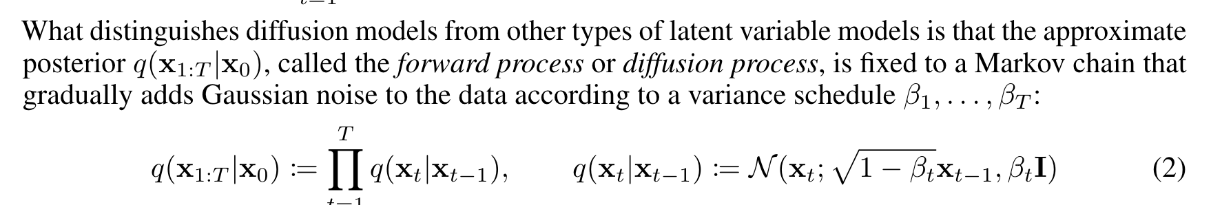
Regarding the forward process:
![]()
I totally get the one extrem of this equation where you’d set beta_t to 1 resulting in an image that is pure noise with a mean of 0 and a variance of 1 like Jeremy explained in lesson 19. However, I don’t understand how (2) would be a normally distributed function for a beta_t that would be close to zero? So the closer we would get to the original image - without noise, or with a very small amount of noise - the “further away” it would be of a normally distributed function, wouldn’t it? How does equation (2) guarantee to be normally distributed if we are very close to the starting point x_0 of the forward diffusion?
Another thing that surprises me in equation (2) is that it is displaying a conditional probability (x_t is happening momentarily under the condition that x_t-1 happened right before), but in (2) the mean for x_t | x_t-1 only seems to be dependent on x_t-1? For two random variables that are jointly normal this
would be the mathematical representation for the conditional probability. (source: https://handoutset.com/wp-content/uploads/2022/05/Probability-Random-Variables-and-Stochastic-Processes-Athanasios-Papoulis-S.-Unnikrishna-Pillai.pdf)
Gaussian noise surely is a normally distributed random variable. But like pointed out before, I don’t think that the images x_0 that are used for the forward diffusion are all normally distributed? So how can equation (2) be jointly normally distributed at all for a beta_t close to 0? Maybe I am reading the equation badly because of the semicolon in the middle after x_t? That notation confuses me a lot to be honest because I don’t know if it is describing just one random variable or two at the same time … Also irritating: for normally distributed random variables usually there are exponential functions all over the place, but these papers don’t display those at all?
Regarding the reverse, generating process:
So like Tanishq pointed out in lesson 19 epsilon is a normally distributed function with a mean of 0 and a variance of 1 and epsilon_θ is equivalent to:
![]()
Like you’ve explained in lesson 19, equation (4) is trained as a neural network. Meaning that it gives an estimate for the noise in the image x_t. So far everything makes sense. But why would we now subtract that estimate from “epsilon ~ N (0,1)”? Doesn’t “~ N (0,1)” imply that epsilon is just pure noise or at least it would imply to be a normally distributed function? So here occurs the same confusion like in the forward process: the closer we get to the original image x_0 the less we could assume to be having a mean of 0 and a variance of 1. Wouldn’t epsilon need to be also somewhat near to the momentary x_t value? And wouldn’t it then have a mean ≠ 0 and a variance ≠ 1 the closer we get to x_0?
Would be awesome to precisely understand all this math stuff. Maybe someone can recommend any mathematically detailed video / paper to dive deeper into all the formulas behind this.
I have to admit I am having a little bit of issue following. I think I see a little that I can address though.
For…
\mathcal{N}(x_t;\sqrt{1-\beta_t}x_{t-1},\beta_t I)
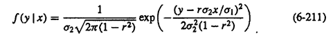
The \mathcal{N}(x_t;\mu,\sigma^2) is referring to the normal distribution, where \mu and \sigma determine the mean and standard deviation. This function is hiding all the math-y bits like the exponential.
\mathcal{N}(\mu,\sigma^2)=\frac{1}{\sigma\sqrt{2\pi}}e^{-\frac{1}{2}(\frac{x-\mu}{\sigma})^2}
In \mathcal{N}(x_t;\mu,\sigma^2) the x_t is essentially the name of the output of the function, or assigning the output of N to the variable x_t
So what happens when \beta_t=0?
We get…
q(x_t|x_{t-1}):=\mathcal{N}(x_t;\sqrt{1-\beta_t}x_{t-1},\beta_t I)
q(x_t|x_{t-1}):=\mathcal{N}(x_t;\sqrt{1-0}x_{t-1},0 I)
q(x_t|x_{t-1}):=\mathcal{N}(x_t;x_{t-1},0)
So, we get a normal distribution with mean \mu=x_{t-1} and standard deviation \sigma=0. Though wait… that isn’t a normal distribution? Actually, it is! A standard normal distribution has a mean \mu=0 and standard deviation \sigma=1, a normal distributiuon is essentially a bell curve that can have any mean and standard deviation.
When \beta_t\approx 0 then q(x_t|x_{t-1}):=\mathcal{N}(x_t;x_{t-1}, \sim 0)\approx x_{t-1}, essentially we are centered at a mean of the previous image, with a no standard deviation! So we just return the input.
(using \sim as plugging in 0 means dividing by zero)
Next the \epsilon bit
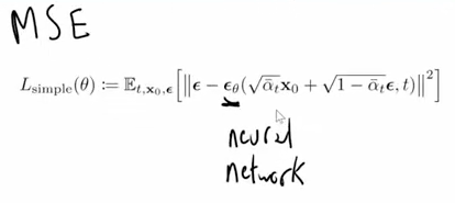
This is the loss function:
L_{simple}(\theta) := \mathbb{E}[\| \epsilon - \epsilon_\theta(\sqrt{\bar\alpha_t}x_0+\sqrt{1-\bar\alpha_t}\epsilon,t) \|^2]
What does a model need to do to be perfectly trained? It needs its loss to be 0! Well, for this loss function as it can’t go negative due to \| ... \|^2. So, how can it do that?
Well lets say \epsilon_\theta returns \epsilon. Then we get…
L_{simple}(\theta) := \mathbb{E}[\| \epsilon - \epsilon \|^2]
L_{simple}(\theta) := \mathbb{E}[\| 0 \|^2]
L_{simple}(\theta) := 0
Okay, so our model needs to predict \epsilon, which is standard normal noise. The input to our model is (\sqrt{\bar\alpha_t}x_0+\sqrt{1-\bar\alpha_t}\epsilon,t). This being image+noise=noisy image, with t being the timestep. This input is a normally distributed about x_{t-1}, while the output is a standard normal distribution also known as noise \epsilon.
4 Likes
This helped me a lot, thank you very much for explaining the details!
I was confused because - like you’ve pointed out - I was assuming that all of the distributions are standard normal distributions! Now everything makes a lot more sense!
So if we set beta_t to zero then we get a normal distribution, that has a no standard deviation. Does that imply that the bell curve is very very narrow and has no spread, because the variance σ^2 would be zero, too? So it’s like an impulse that has a probability of 1 for the center (x_t-1) and has no standard deviation and no variance, so the spread is zero? That can be considered as a normally distributed function as well?
Regarding the loss: so like you’ve explained ϵ is standard normal noise and the input ϵ_0 to the model is
Like you’ve said optimally we want to have a loss that gets smaller and smaller, maybe even all the way down as close to zero as possible. But like Jeremy pointed out it would be mathematically impossible to just subtract all the noise at once, which makes total sense. So we subtract it iteratively, right? Maybe someone can explain the procedure of how the first iterations are going from pure noise to some image that still has a lot of noise in it?
If we look at the animation in video 19, at about 01:11:15, it seems like the most difficult part for the generative process would be the first 800 timesteps, going from pure noise to something that has contours which look somewhat similar to a t-shirt.
This reminds me a lot of lesson 9A at 28:00 onwards when Jonathan explained that it is easy to get to pure noise - as it could simply have been created by adding it to every image in the data set until they diffuse into pure noise. But now as we want to walk in the other direction we need to solve those ordinary differential equations that Jonathan talked about. However, in equation (4) of the DDPM paper, ϵ_0 just seems to be trained by using a single image x_0, rather than using all the images ∑ x? Shouldn’t the loss being calculated by moving closer to the manifold like explained in lesson 9A?
Still struggling with the details of the generative process, but I think I get closer every day … seems like I’m reducing my inner knowledge loss, just being like a neural network myself, too lol! Thanks again for your help marii!
1 Like
I have made a few images to illustrate the topics that I’ve written about in my last two posts in this thread. I thought it could be helpful for all the other folks out there struggling with the maths when it comes to diffusion like myself. I thought maybe it could be a good way to demonstrate what kind of signals are processed behind the curtain in a DDPM.
So the basic idea of the presented paper is to focus solely on the mean of the noisy images. Why is that? If we take a closer look at how a normally distributed function moves to the side as the mean increases:
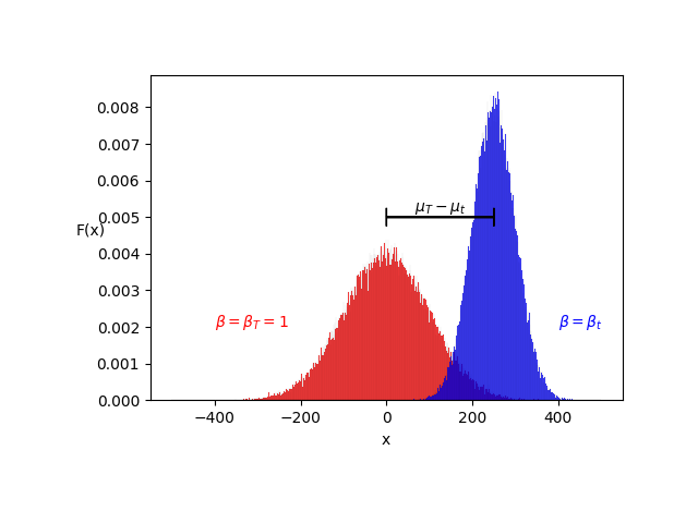
We first of all can see that the function is growing in height because of the higher variance. It is also notable that the mean is traveling along the x-axis for every increase of μ. The neural network in a DDPM now tries to estimate the distance from one mean to the other (μ_T - μ_t). Therefore in the paper they write the formula (14) in that style to show that the neural network tries to guess the actual timestep and then assigns that estimate to the subtraction formula. As the above image shows a function of just two dimensions (F(x) and x) it is just a simplification of the actual math which would compute much more additional dimensions like Jonathan pointed out in lesson 9 it could be up to 200 k dimensions or even more for images that consist of color channels, heigth and width. This is exactly why in the animation of the video in lesson 19 it takes 800 out of 1000 steps to get to the first image that somewhat looks anything like contours of a shirt. To demonstrate the cause of this I’ve made another image:
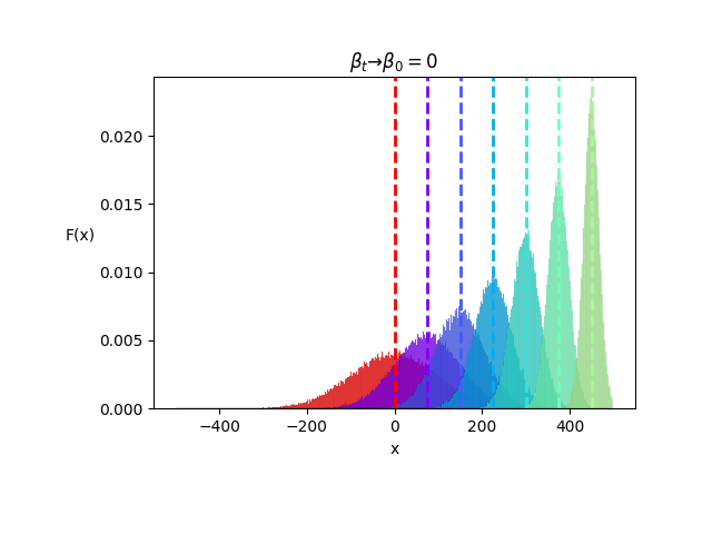
As beta_t is 1 (red) the function is a standard normal distribution. As μ increases and the variance decreases, the means of the distributions get more and more prominent. But for values of beta_t close to one (purple) it is harder to subtract a predicted noise, simply because the functions are very close to each other. I guess that is exactly the reason why the multidimensional SGD / ordinary differential equation solvers can’t produce an estimate that makes a lot of sense at the beginning of the generative process, because of the small changes in μ over all the dimensions. Two conclude all of this I’ve made an image to sum up the two extrem situations:
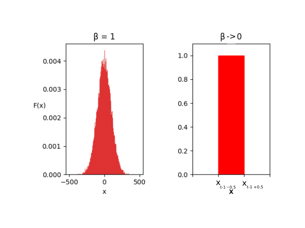
On the right side you can see what I was referring to when I asked if the distribution would become “an impulse” if the variance is zero. I guess the probability could only exist around one point on the x axis (μ = x_t-1) with a total width of 1 on the x-axis so that the density functions squares up to 1. And on the left side you can see the standard normal distribution with 1000 squares / possible values from 0 to T on the x-axis, representing the 1000 timesteps.
Maybe someone can clarify all of this. I hope that I haven’t mixed that up so please correct me if I’ve created the images wrongly! I hope this can be of help to anybody, too though.
1 Like
I stumbled a bit over the part where Jeremy et al talk about new “diffusion like” papers coming out all the time that actually dont do diffusion at all. Johno then coins the term: “iterative refinement”.
I fail to understand what this exactly means:
If apparently these “non diffusion” based approaches still use iterative refinement (which I consider to be anything in which noise is gradually removed) what exactly makes an approach to be in the category of “iterative refinement” and not in the category of “stable diffusion”?
Or in other words, what makes an “iterative refinement” approach to be “stable diffusion”?
I think the term “iterative refinement” just wants to indicate that all the procedures are executed iteratively. Meaning that these kind of algorithms can’t deliver an approximation instantly. (e.g. like explained by Johno in Lesson 9A you can’t just subtract all the noise at once in a DDPM, you have to go step by step, iteratively refining the noisy images until, after the last iteration, the distribution of the final result will be as close to the sum of original data points as possible.)
The terms diffusion, stable diffusion and linear diffusion all have their origin in the DDPM paper discussed in the lesson. In all of these models the data is iteratively covered with white gaussian noise until the data finally diffuses completely resulting in just pure white gaussian noise. The generative process then starts by subtracting a bit of that pure noise step by step, refining the signal iteratively to generate a desired result as close to the sum of all data points that were used in training.
However it would also be possible to diffuse the data into something other than white gaussian noise, for example a so called gamma function (I’ve seen this in this paper: https://arxiv.org/pdf/2106.07582.pdf). So here the terminologies start to get really confusing because DDPMs always use white gaussian noise. So I guess you could go back in time to the original thermodynamics paper of 2015 that was kind of the inspiration for the 2020 DDPM paper. In the 2015 thermodynamics paper they classified this diffusion process by stating that it is “destroying” the original data distributions. So in a diffusion model your data always gets “destroyed” somehow. It could be white noise, pink noise, a mixture of noises, a gamma function. The basic idea is just to add so much of it to the original data until it diffuses into it.
However, Iterative refinement is a great terminology because it includes other models as well that do not destroy their data distributions. For example generative adversarial networks (GAN) or variational autoencoders (VAE) (Variational Autoencoder in TensorFlow (Python Code)). An variational autoencoder for example does not diffuse its data into noise or any other signal. To simplify one could say that an encoder inside a VAE is kind of compressing its data into a more compact representation of itself in form of a latent vector. The decoder then iteratively tries to refine that compressed data into a representation as close to the data that was being encoded. So the generative idea is similar but the data does not diffuse here in these models.
There are also a lot of other additional approaches and techniques out there that could be listed here as well. As it is a very young research field there will follow a lot of publications in the next few decades. They’ll maybe all have different implementations and are technically subclasses of something else but in order to form a superordinate class of all these procedures, the term iterative refinement is a very good fit I think.
2 Likes
Thanks for your answer @Laulito, I think indeed it comes down to what you say. Yesterday I came across this passage, which I assume to be “the definition”:
I am trying to implement the sample method from DDPM, but I can’t seem to track back the steps taken in @ilovescience notebook (15_DDPM) to the paper. In the paper I can only find the “Algorithm 2” description, which I followed but it seems to be a bit different from what is done in 15_DDPM.
Has anybody been able to understand these steps in detail?
EDIT: I wasn’t able to confirm the expressions are identical mathematically (![]() ), but I guess they are. At least both of them give similar result in terms of samples. I suspect Tanishk rewrote the expression from the paper to the form of the notebook to show that the result x_t is a weighted average of the prediction for x_0 and the previous timestep x_t_1 (plus new noise)
), but I guess they are. At least both of them give similar result in terms of samples. I suspect Tanishk rewrote the expression from the paper to the form of the notebook to show that the result x_t is a weighted average of the prediction for x_0 and the previous timestep x_t_1 (plus new noise)
1 Like
In the start of this lesson, Jeremy gave a homework to implement Dropout2d - I have taken a shot at it. Here is the code below.
#reference - https://discuss.pytorch.org/t/what-is-the-difference-between-nn-dropout2d-and-nn-dropout/108192
class Dropout2D(nn.Module):
    def __init__(self, p=0.1):
        super().__init__()
        self.p = p

    def forward(self, x):
        if not self.training:
            return x

        N, C, H, W = x.size()

        dist = distributions.binomial.Binomial(tensor(1.0).to(x.device), probs=1-self.p)

        mask = dist.sample((N,C,H,W)) * (1/(1-self.p))

        return x * mask
Any feedback for if this is the right implementation is welcome!
Hi Tanisq @ilovescience, thanks a lot for all the hard work. Seriously impressive what you all put out for us.
Had a quick question related to what @johnri99 asked at the beginning of the year (never too late!), i.e. why do you use this definition of mu_t? Whereas the Sampling algorithm (algorithm) leverages something that, to me, looks a lot simpler, which is also found in eq 11:
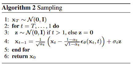
In other words: what didn’t we ‘simply’ follow the algorithm outlined by the authors? I tried it and it seems to work. But I feel like I’m missing something… Thanks in advance ![]()
2 Likes
Hi @anirudh15 , I think .sample along all the 4 dimensions of N,C,H,W would set random values within the generated distributions to 0 but not entire feature maps of a channel to 0. Doing the following would be better
shape = x.size()
masks = distributions.binomial.Binomial(tensor(1.0).to(x.device), probs=1-self.p)
dist = masks.sample(shape[:2])
return x * dist * (1/(1-self.p))
With this modification, entire feature maps of a channel will be set to zero with the specified probability. The shape[:2] is used to generate binary masks for each channel independently.
Hey @Laulito, did you ever get a better explanation of what’s happening in this process? As I glanced at your pictures of these distributions, I thought more and more that basically every pixel has a 1000 normal distributions from t=0->1000. I’m still not clear on what is happening in this algorithm.
Side note: I’m really struggling to read these papers. I was only taught up to Linear Stochastic Models in Elec. Eng bachelors course 10 years ago. Is this level of difficulty expected?
In all of the diagrams that I drew there was only one dimension x. That was a very brutal simplification to try to graphically show what is happening in diffusion like algorithms. But in reality rather than using just one dimension the calculations are constructed by stochastic processes like markov chains that are mathematically described by joint probability density functions with various dimensions.
To give an explanation that gets more precise about the whole magic behind generative ai you could describe the whole process like this: If you’ve got 3 colour channels from an RGB video or image signal you always have 3 values for every pixel. One value for red, one for green, one for blue. Say you’d wanted to find out if changing the RGB values of a certain pixel of an image by hand was reducing the generative ai / diffusion / iterative refinement loss calculations or not. Then with this task at hand you would never know if increasing blue and reducing green while reducing red at the same time would reduce the loss more drastically like increasing blue, reducing green while increasing red. Or increasing red, reducing blue while increasing green. Now at this point we are only taking into account the three colour values of the RGB signal. But actually the loss depends on every pixel relatively to each other, too so we get a whole lot of additional dimensions as well.
If you try to think of it in pixels again: Say your diffusion model has to generate images of a house in front of a lake. Now for some of the generated images blue might be in the bottom left corner and for some blue might be in the bottom right corner DEPENDING TOTALLY on the positions and values of every other colour pixel in the image relatively to each other. Each and every probability distribution of all of the images that we use for training is combined and that creates a joint probability distribution that spans a certain multidimensional area from which you can sample later after reducing the loss as much as possible.
I hope this was pointed out understandably and correct me anytime if I’m wrong guys. I hope all of this can be of help to anybody who tries to do the course and struggles with understanding the algorithms at first glance. I hope through brisk exchange in threads like this the precise mathematical description of stochastic problems like markov chains can be explained with words and models to get the imagination inside the brains going and help deepen the understanding of it all.
Thanks for explaining what’s happening here. I somewhat abstractly understand you. However, I think I have to go look up an example of a single or dual layer Neural Network where it’s inputs are fed by a RGB image, and this example shows how the probability distributions are developed/changed from beginning to the end of the model.
The neural network takes the actual RGB pixels as input neurons when it is training with the dataset. After let’s say 30 epochs it reduced the KL divergences meaning it reduced the loss and has set the weights from now on. Now you have a pretrained model with weights that are already set and that allows you to sample form it and generate RGB images by sampling from said joint probability distribution from my last reply. It is like a multidimensional space that is stretched over the united composite set if you want to imagine it visually. And that’s why generative ai models like diffusion models can create so seemingly endless variations of the same image because from a mathematical point of view there are just so many dimensions that the possible combinations of three colour values for maybe every 256x256 = 65536 pixel relatively to each other are literally almost endless. The noisy images that are initialised first carry a lot of information from an information theory point of view because they are “rich in information”. After increasing the noise in the forward process on a lot of images you can decrease the noise in the generative process from “many angles”. Images starting from different corners or being mirrored - all of these pixel combinations need be reachable by subtracting the noise iteratively.
Keep in mind though that this is still all a little bit simplified because in the papers a lot of times they need to kind of use some kind of mathematical tricks and tools to make these horrible stochastic equations somehow solvable. But that’s the point where I’m a bit lost still when it’s about the details of the details. Step by step I need to be patient with myself. ![]()