Lesson 19 official topic

oops, missed it. No problem, I will watch the recorded video.
Regarding last lesson, in Jupyter Notebook if you use latex math like \alpha and hit TAB, it will transform it to the corresponding UTF char.

3 Likes

This issue persists in the latest version. The problem seems to be that the __init__ method for the DDPMCB class isn’t running super().__init__(). Adding this line fixes the issue.

2 Likes

Many thanks - will fix now.

1 Like

Training the UNet fails on an M1 Mac, as group normalisation seems to not yet be implemented for the MPS device. Falling back to CPU (using PYTORCH_ENABLE_MPS_FALLBACK=1) causes the Python process to crash.

I may have to run the notebooks on Colab rather than locally.

1 Like

Trying to follow the original paper for the sampling process I am struggling to see how the xo and xt coefficients are derived. I can see that x_0_hat corresponds to equation 15 in the paper and is a way to get to x0 in one step. I was expecting that the x0 and xt coefficients would follow the equation in step 4 of the sampling (Algorithm 2) in the same way that the training stage follows Algorithm 1, however, it doesn’t seem to. As mentioned in the lesson, instead it takes a weighted average of the predicted x0 and the current xt. I understand this but can’t see where the calculation of the coefficients comes from.

Probably me not understanding the paper well enough but if anybody can help explain it would be great

The coefficients come from the equation for q(\mathbf{x}_{t-1} | \mathbf{x}_{t}, \mathbf{x}_{0}):


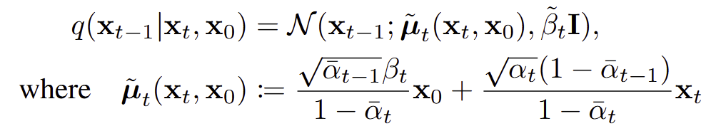
What this equation tells us is how \mathbf{x}_{t-1} is distributed given \mathbf{x}_0 (which we get an estimate of) and \mathbf{x}_{t}.

The loss function math demonstrates that the mean of our reverse process distribution should match the mean of q(\mathbf{x}_{t-1} | \mathbf{x}_{t}, \mathbf{x}_{0}) :

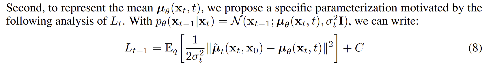
Therefore, our model must learn to predict \tilde{\mathbf{\mu}}_t, which it does by predicting the noise to remove from \mathbf{x}_t to get an estimate of \mathbf{x}_0 which we plug into that equation for to finally get our mean \tilde{\mathbf{\mu}}_t for q(\mathbf{x}_{t-1} | \mathbf{x}_{t}, \mathbf{x}_{0}).

Hope this is clear! Let me know if you have any other questions!

3 Likes

Thanks Tanishq, I can see where the coefficients come from now but I am still struggling with the interpretation. I can see from equation 7 in the paper that what you are generating as x_t in the code is equivalent to the calculated \tilde{\mu}_t(x_t,x_0) plus the standard deviation at that time step multiplied by the generated random noise. I am not sure why this can then be interpreted as x_{t-1}?

Great lesson again thanks everyone. Is it just me or is the audio for the great explanation by @ilovescience (Inheriting from miniai TrainCB onwards) a bit dodgy?

It’s not just you. I’ve been nagging Tanishq about upgrading his mic setup so this feedback is most helpful! :wink:

2 Likes

The n_inp issue is still presented in course22p2/15_DDPM.ipynb at master · fastai/course22p2 · GitHub

class DDPMCB should have super().__init__()

Thanks for the reminder - just pushed that change.

Sorry for disturbing, but super().__init__() still not in DDPMCB.

Oh there’s 2 versions of it - in NBs 15 and 17. I’d only changed 15. I’ve changed 17 now.

Hello Team,

Many thanks for this wonderful video series. I am learning a lot from it. I’m facing an issue with loading the fashion mnist dataset in the 15_DDPM.ipynb. Following are the details.

When I run the code,

set_seed(42)
bs = 128
tds = dsd.with_transform(transformi)
dls = DataLoaders.from_dd(tds, bs, num_workers=1)

dt = dls.train
xb,yb = next(iter(dt))
xb.shape,yb[:10]

I get the following error,

---------------------------------------------------------------------------
AttributeError                            Traceback (most recent call last)
Cell In[7], line 8
      5 # dls = torch_dataloader(tds, bs, num_workers=1)
      7 dt = dls.train
----> 8 xb,yb = next(iter(dt))
      9 xb.shape,yb[:10]

File T:\installations\anaconda\envs\3d_env\lib\site-packages\torch\utils\data\dataloader.py:441, in DataLoader.__iter__(self)
    439     return self._iterator
    440 else:
--> 441     return self._get_iterator()

File T:\installations\anaconda\envs\3d_env\lib\site-packages\torch\utils\data\dataloader.py:388, in DataLoader._get_iterator(self)
    386 else:
    387     self.check_worker_number_rationality()
--> 388     return _MultiProcessingDataLoaderIter(self)

File T:\installations\anaconda\envs\3d_env\lib\site-packages\torch\utils\data\dataloader.py:1042, in _MultiProcessingDataLoaderIter.__init__(self, loader)
   1035 w.daemon = True
   1036 # NB: Process.start() actually take some time as it needs to
   1037 #     start a process and pass the arguments over via a pipe.
   1038 #     Therefore, we only add a worker to self._workers list after
   1039 #     it started, so that we do not call .join() if program dies
   1040 #     before it starts, and __del__ tries to join but will get:
   1041 #     AssertionError: can only join a started process.
-> 1042 w.start()
   1043 self._index_queues.append(index_queue)
   1044 self._workers.append(w)

File T:\installations\anaconda\envs\3d_env\lib\multiprocessing\process.py:121, in BaseProcess.start(self)
    118 assert not _current_process._config.get('daemon'), \
    119        'daemonic processes are not allowed to have children'
    120 _cleanup()
--> 121 self._popen = self._Popen(self)
    122 self._sentinel = self._popen.sentinel
    123 # Avoid a refcycle if the target function holds an indirect
    124 # reference to the process object (see bpo-30775)

File T:\installations\anaconda\envs\3d_env\lib\multiprocessing\context.py:224, in Process._Popen(process_obj)
    222 @staticmethod
    223 def _Popen(process_obj):
--> 224     return _default_context.get_context().Process._Popen(process_obj)

File T:\installations\anaconda\envs\3d_env\lib\multiprocessing\context.py:336, in SpawnProcess._Popen(process_obj)
    333 @staticmethod
    334 def _Popen(process_obj):
    335     from .popen_spawn_win32 import Popen
--> 336     return Popen(process_obj)

File T:\installations\anaconda\envs\3d_env\lib\multiprocessing\popen_spawn_win32.py:93, in Popen.__init__(self, process_obj)
     91 try:
     92     reduction.dump(prep_data, to_child)
---> 93     reduction.dump(process_obj, to_child)
     94 finally:
     95     set_spawning_popen(None)

File T:\installations\anaconda\envs\3d_env\lib\multiprocessing\reduction.py:60, in dump(obj, file, protocol)
     58 def dump(obj, file, protocol=None):
     59     '''Replacement for pickle.dump() using ForkingPickler.'''
---> 60     ForkingPickler(file, protocol).dump(obj)

AttributeError: Can't pickle local object 'inplace.<locals>._f'

I’m stuck after many tries. Please help.

Solution for the above issue.

I didn’t mention which OS I was running things on. I’m using Windows 11. There seems a problem with Pickle, multiple processes, and Windows. See this thread - Can't pickle local object 'DataLoader.__init__.<locals>.<lambda>' - #24 by asura - vision - PyTorch Forums

Changing,

dls = DataLoaders.from_dd(tds, bs, num_workers=1) to dls = DataLoaders.from_dd(tds, bs) helped me solve the issue.

2 Likes

Here is my code to upsample the less noisier samples:

def noisify(x0, ᾱ, upsample=False, upsample_p=0.7, undersample_i=700):
    device = x0.device
    n = len(x0)
    if upsample:
        upsample = torch.bernoulli(torch.ones((n,))*upsample_p).bool()
        t_under = torch.randint(0, undersample_i, (n,), dtype=torch.long)
        t_up = torch.randint(undersample_i, n_steps, (n,), dtype=torch.long)
        t = torch.where(upsample, t_up, t_under)
    else:
        t = torch.randint(0, n_steps, (n,), dtype=torch.long)
    ε = torch.randn(x0.shape, device=device)
    ᾱ_t = ᾱ[t].reshape(-1, 1, 1, 1).to(device)
    xt = ᾱ_t.sqrt()*x0 + (1-ᾱ_t).sqrt()*ε
    return (xt, t.to(device)), ε

Hey guys, I also struggle understanding the forward and the reverse process mathematically. Would be awesome to understand the details better, maybe someone can help me out.

Regarding the forward process:
Bildschirmfoto 2023-09-25 um 15.27.47

I totally get the one extrem of this equation where you’d set beta_t to 1 resulting in an image that is pure noise with a mean of 0 and a variance of 1 like Jeremy explained in lesson 19. However, I don’t understand how (2) would be a normally distributed function for a beta_t that would be close to zero? So the closer we would get to the original image - without noise, or with a very small amount of noise - the “further away” it would be of a normally distributed function, wouldn’t it? How does equation (2) guarantee to be normally distributed if we are very close to the starting point x_0 of the forward diffusion?

Another thing that surprises me in equation (2) is that it is displaying a conditional probability (x_t is happening momentarily under the condition that x_t-1 happened right before), but in (2) the mean for x_t | x_t-1 only seems to be dependent on x_t-1? For two random variables that are jointly normal this

Bildschirmfoto 2023-09-25 um 15.49.06

would be the mathematical representation for the conditional probability. (source: https://handoutset.com/wp-content/uploads/2022/05/Probability-Random-Variables-and-Stochastic-Processes-Athanasios-Papoulis-S.-Unnikrishna-Pillai.pdf)

Gaussian noise surely is a normally distributed random variable. But like pointed out before, I don’t think that the images x_0 that are used for the forward diffusion are all normally distributed? So how can equation (2) be jointly normally distributed at all for a beta_t close to 0? Maybe I am reading the equation badly because of the semicolon in the middle after x_t? That notation confuses me a lot to be honest because I don’t know if it is describing just one random variable or two at the same time … Also irritating: for normally distributed random variables usually there are exponential functions all over the place, but these papers don’t display those at all?

Regarding the reverse, generating process:

Bildschirmfoto 2023-09-25 um 17.18.53

So like Tanishq pointed out in lesson 19 epsilon is a normally distributed function with a mean of 0 and a variance of 1 and epsilon_θ is equivalent to:

Bildschirmfoto 2023-09-25 um 17.23.49

Like you’ve explained in lesson 19, equation (4) is trained as a neural network. Meaning that it gives an estimate for the noise in the image x_t. So far everything makes sense. But why would we now subtract that estimate from “epsilon ~ N (0,1)”? Doesn’t “~ N (0,1)” imply that epsilon is just pure noise or at least it would imply to be a normally distributed function? So here occurs the same confusion like in the forward process: the closer we get to the original image x_0 the less we could assume to be having a mean of 0 and a variance of 1. Wouldn’t epsilon need to be also somewhat near to the momentary x_t value? And wouldn’t it then have a mean 0 and a variance 1 the closer we get to x_0?

Would be awesome to precisely understand all this math stuff. Maybe someone can recommend any mathematically detailed video / paper to dive deeper into all the formulas behind this.

I have to admit I am having a little bit of issue following. I think I see a little that I can address though.

For…
\mathcal{N}(x_t;\sqrt{1-\beta_t}x_{t-1},\beta_t I)
The \mathcal{N}(x_t;\mu,\sigma^2) is referring to the normal distribution, where \mu and \sigma determine the mean and standard deviation. This function is hiding all the math-y bits like the exponential.
\mathcal{N}(\mu,\sigma^2)=\frac{1}{\sigma\sqrt{2\pi}}e^{-\frac{1}{2}(\frac{x-\mu}{\sigma})^2}

In \mathcal{N}(x_t;\mu,\sigma^2) the x_t is essentially the name of the output of the function, or assigning the output of N to the variable x_t

So what happens when \beta_t=0?

We get…
q(x_t|x_{t-1}):=\mathcal{N}(x_t;\sqrt{1-\beta_t}x_{t-1},\beta_t I)
q(x_t|x_{t-1}):=\mathcal{N}(x_t;\sqrt{1-0}x_{t-1},0 I)
q(x_t|x_{t-1}):=\mathcal{N}(x_t;x_{t-1},0)
So, we get a normal distribution with mean \mu=x_{t-1} and standard deviation \sigma=0. Though wait… that isn’t a normal distribution? Actually, it is! A standard normal distribution has a mean \mu=0 and standard deviation \sigma=1, a normal distributiuon is essentially a bell curve that can have any mean and standard deviation.

When \beta_t\approx 0 then q(x_t|x_{t-1}):=\mathcal{N}(x_t;x_{t-1}, \sim 0)\approx x_{t-1}, essentially we are centered at a mean of the previous image, with a no standard deviation! So we just return the input.

(using \sim as plugging in 0 means dividing by zero)

Next the \epsilon bit

This is the loss function:
L_{simple}(\theta) := \mathbb{E}[\| \epsilon - \epsilon_\theta(\sqrt{\bar\alpha_t}x_0+\sqrt{1-\bar\alpha_t}\epsilon,t) \|^2]
What does a model need to do to be perfectly trained? It needs its loss to be 0! Well, for this loss function as it can’t go negative due to \| ... \|^2. So, how can it do that?

Well lets say \epsilon_\theta returns \epsilon. Then we get…
L_{simple}(\theta) := \mathbb{E}[\| \epsilon - \epsilon \|^2]
L_{simple}(\theta) := \mathbb{E}[\| 0 \|^2]
L_{simple}(\theta) := 0
Okay, so our model needs to predict \epsilon, which is standard normal noise. The input to our model is (\sqrt{\bar\alpha_t}x_0+\sqrt{1-\bar\alpha_t}\epsilon,t). This being image+noise=noisy image, with t being the timestep. This input is a normally distributed about x_{t-1}, while the output is a standard normal distribution also known as noise \epsilon.

3 Likes

This helped me a lot, thank you very much for explaining the details!

I was confused because - like you’ve pointed out - I was assuming that all of the distributions are standard normal distributions! Now everything makes a lot more sense!

So if we set beta_t to zero then we get a normal distribution, that has a no standard deviation. Does that imply that the bell curve is very very narrow and has no spread, because the variance σ^2 would be zero, too? So it’s like an impulse that has a probability of 1 for the center (x_t-1) and has no standard deviation and no variance, so the spread is zero? That can be considered as a normally distributed function as well?

Regarding the loss: so like you’ve explained ϵ is standard normal noise and the input ϵ_0 to the model is

Like you’ve said optimally we want to have a loss that gets smaller and smaller, maybe even all the way down as close to zero as possible. But like Jeremy pointed out it would be mathematically impossible to just subtract all the noise at once, which makes total sense. So we subtract it iteratively, right? Maybe someone can explain the procedure of how the first iterations are going from pure noise to some image that still has a lot of noise in it?

If we look at the animation in video 19, at about 01:11:15, it seems like the most difficult part for the generative process would be the first 800 timesteps, going from pure noise to something that has contours which look somewhat similar to a t-shirt.

This reminds me a lot of lesson 9A at 28:00 onwards when Jonathan explained that it is easy to get to pure noise - as it could simply have been created by adding it to every image in the data set until they diffuse into pure noise. But now as we want to walk in the other direction we need to solve those ordinary differential equations that Jonathan talked about. However, in equation (4) of the DDPM paper, ϵ_0 just seems to be trained by using a single image x_0, rather than using all the images ∑ x? Shouldn’t the loss being calculated by moving closer to the manifold like explained in lesson 9A?

Still struggling with the details of the generative process, but I think I get closer every day … seems like I’m reducing my inner knowledge loss, just being like a neural network myself, too lol! Thanks again for your help marii!

I have made a few images to illustrate the topics that I’ve written about in my last two posts in this thread. I thought it could be helpful for all the other folks out there struggling with the maths when it comes to diffusion like myself. I thought maybe it could be a good way to demonstrate what kind of signals are processed behind the curtain in a DDPM.

So the basic idea of the presented paper is to focus solely on the mean of the noisy images. Why is that? If we take a closer look at how a normally distributed function moves to the side as the mean increases:

MuT minus Mut

We first of all can see that the function is growing in height because of the higher variance. It is also notable that the mean is traveling along the x-axis for every increase of μ. The neural network in a DDPM now tries to estimate the distance from one mean to the other (μ_T - μ_t). Therefore in the paper they write the formula (14) in that style to show that the neural network tries to guess the actual timestep and then assigns that estimate to the subtraction formula. As the above image shows a function of just two dimensions (F(x) and x) it is just a simplification of the actual math which would compute much more additional dimensions like Jonathan pointed out in lesson 9 it could be up to 200 k dimensions or even more for images that consist of color channels, heigth and width. This is exactly why in the animation of the video in lesson 19 it takes 800 out of 1000 steps to get to the first image that somewhat looks anything like contours of a shirt. To demonstrate the cause of this I’ve made another image:

beta_to_0

As beta_t is 1 (red) the function is a standard normal distribution. As μ increases and the variance decreases, the means of the distributions get more and more prominent. But for values of beta_t close to one (purple) it is harder to subtract a predicted noise, simply because the functions are very close to each other. I guess that is exactly the reason why the multidimensional SGD / ordinary differential equation solvers can’t produce an estimate that makes a lot of sense at the beginning of the generative process, because of the small changes in μ over all the dimensions. Two conclude all of this I’ve made an image to sum up the two extrem situations:

beta 0 and 1

On the right side you can see what I was referring to when I asked if the distribution would become “an impulse” if the variance is zero. I guess the probability could only exist around one point on the x axis (μ = x_t-1) with a total width of 1 on the x-axis so that the density functions squares up to 1. And on the left side you can see the standard normal distribution with 1000 squares / possible values from 0 to T on the x-axis, representing the 1000 timesteps.

Maybe someone can clarify all of this. I hope that I haven’t mixed that up so please correct me if I’ve created the images wrongly! I hope this can be of help to anybody, too though.

I stumbled a bit over the part where Jeremy et al talk about new “diffusion like” papers coming out all the time that actually dont do diffusion at all. Johno then coins the term: “iterative refinement”.

I fail to understand what this exactly means:

If apparently these “non diffusion” based approaches still use iterative refinement (which I consider to be anything in which noise is gradually removed) what exactly makes an approach to be in the category of “iterative refinement” and not in the category of “stable diffusion”?

Or in other words, what makes an “iterative refinement” approach to be “stable diffusion”?